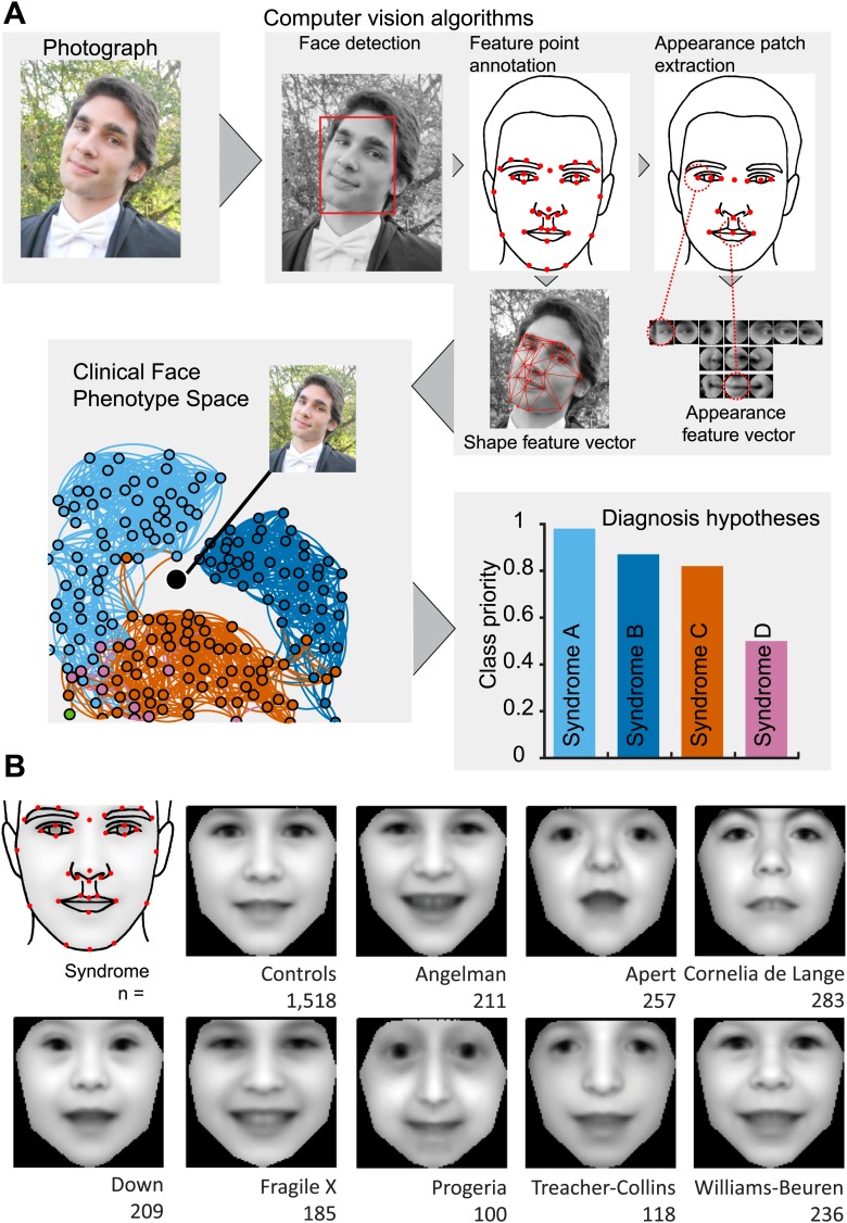
Figure 1. Overview of the computational approach and average faces of syndromes.

(A) A photo is automatically analyzed to detect faces and feature points are placed using computer vision algorithms. Facial feature annotation points delineate the supra-orbital ridge (8 points), the eyes (mid points of the eyelids and eye canthi, 8 points), nose (nasion, tip, ala, subnasale and outer nares, 7 points), mouth (vermilion border lateral and vertical midpoints, 6 points) and the jaw (zygoma mandibular border, gonion, mental protrubance and chin midpoint, 7 points). Shape and Appearance feature vectors are then extracted based on feature points and these determine the photo's location in Clinical Face Phenotype Space (further details on feature points in Figure 1—figure supplement 1). This location is then analyzed in the context of existing points in Clinical Face Phenotype Space to extract phenotype similarities and diagnosis hypotheses (further details on Clinical Face Phenotype Space with simulation examples in Figure 1—figure supplement 2). (B) Average faces of syndromes in the database constructed using AAM models (‘Materials and methods’) and number of individuals which each average face represents. See online version of this manuscript for animated morphing images that show facial features differing between controls and syndromes (Figure 2).

DOI:http://dx.doi.org/10.7554/eLife.02020.003

Figure 1—figure supplement 1.

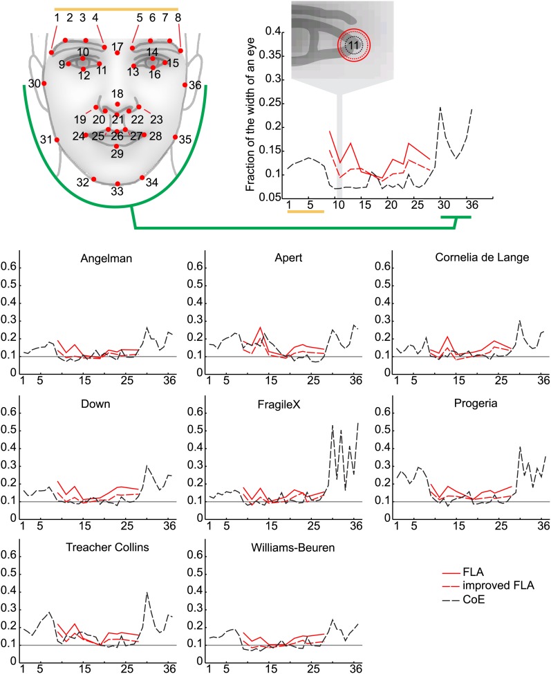
(A) The 36 facial feature points annotated by the automatic image analysis algorithm. Supra-orbital ridge (8 points), the eyes (mid points of the eyelids and eye canthi, 8 points), nose (nasion, tip, ala, subnasale and outer nares, 7 points), mouth (vermilion border lateral and vertical midpoints, 6 points), and the jaw (zygoma mandibular border, gonion, mental protrubance and chin midpoint, 7 points). (B) The annotation accuracies relative to the manually annotated ground truth of each of the computer vision modules. Points 1–8 refer to the supra-orbital ridge, points 30–36 refer to the jaw points. Accuracies for the points annotated by the modules FLA, improved FLA and CoE are shown for each syndrome and control groups. Accuracies are shown as the average error relative to the width of an eye.

DOI:http://dx.doi.org/10.7554/eLife.02020.004

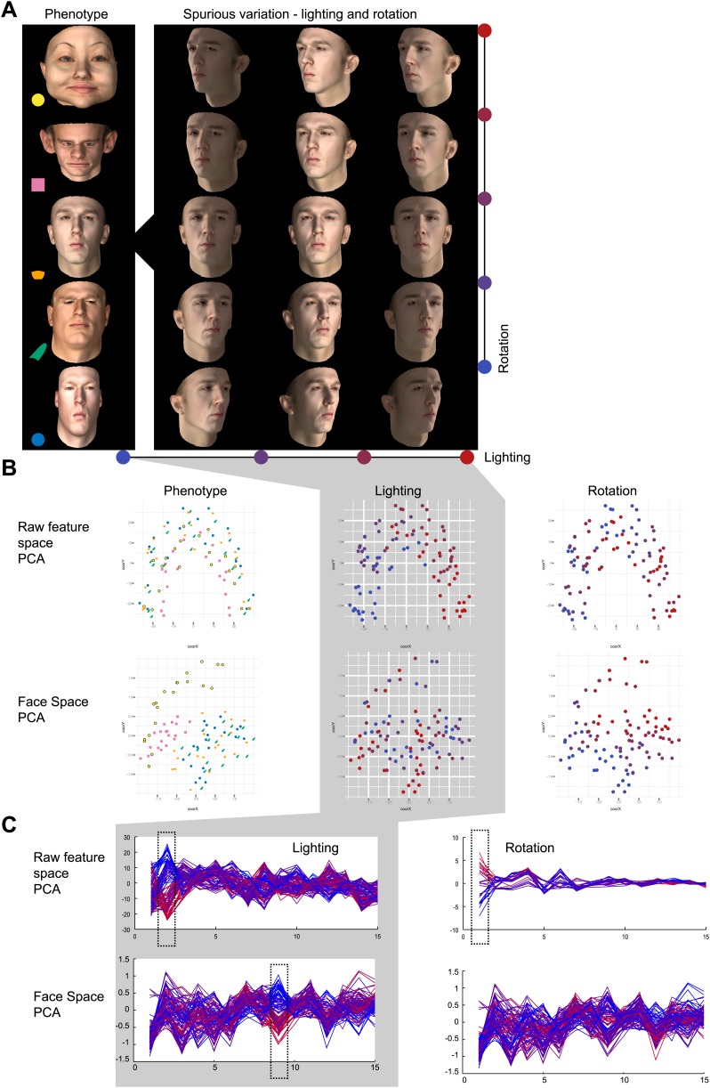
Figure 1—figure supplement 2. Phenotypic vs spurious feature variation in Clinical Face Phenotype Space using simulated faces.

Simulated 3D faces were used to visualize the influence of spurious variation in raw feature space and Clinical Face Phenotype Space. (A) 100 faces with controlled phenotype, lighting, and rotation variation were rendered. (B) Visualization of a population of simulated faces in the first two Multi-Dimensional Scaling (MDS) modes. Face clustering in raw feature space and Clinical Face Phenotype Space colored by lighting, rotation, and face phenotype, respectively. In the raw feature space lighting is the dominating clustering factor, in Clinical Face Phenotype Space phenotype underlies the primary clustering. (C) The first 16 modes of PCA decomposition of the raw feature vectors and in the Clinical Face Phenotype Space colored by lighting and rotation of the simulated faces. In the raw feature space, lighting, and rotation variation are encoded in the 2nd and 1st modes, indicating that clustering is dominated by spurious variation. In the Clinical Face Phenotype Space, lighting is represented in the 9th mode, whereas rotation is no longer represented in the first 16 modes. This shows that the Clinical Face Phenotype Space transformation reduces the influence of spurious variation on clustering of phenotypes.

DOI:http://dx.doi.org/10.7554/eLife.02020.005