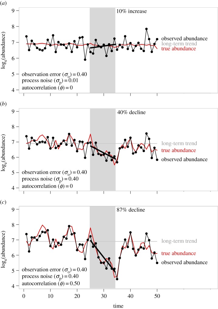
Figure 1.

Three example hypothetical stable time series of abundance (no true underlying time trend) with a starting abundance of 1000 individuals (horizontal grey line). The time series in each panel were generated by setting density-dependence (b in equation (2.1)) to 0.65 and the population growth rate (λ) to 2.4. Variability in the true and observed time series is solely a function of lag-1 autocorrelated (ϕ) process noise (∼N(0, σ_p)) and observation error (∼N(0, σ_o)), the latter only for the observed time series; see lower left corner of each panel for values of these parameters. Closed circles and thin black line are observed abundance, whereas the red line without symbols is the underlying true stochastic abundance (state). The thick black lines are least-square linear regressions of the relationship between log_e abundance and time for time steps 25–34; the corresponding estimated per cent change in raw abundance over the 10 years is shown at the top of panels (a–c). These panels illustrate that despite a long-term stable trend in abundance, quantifying trends in abundance over short time scales may lead to falsely classifying the population as decreasing in abundance, especially at high magnitudes of process noise (b,c), and lag-1 autocorrelation in process noise (c).