
Fig. 5.
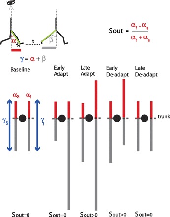
Schematic of spatial changes occurring throughout adaptation. Stick figures at top show the sagittal view of someone walking on the treadmill. The limb angle at heel-strike (i.e., α) is shown at a time period t before the limb angle is at toe-off (i.e., β). Eye icon indicates that diagrams below the sagittal schematic represent the bird's-eye view of the subject stepping on the treadmill. Lines in the bird's-eye view are projections of limb motions during stance at different points in the experimental paradigm. Trunk position is represented by black circles. Red and gray lines represent limb axis projection at angles α and β. Blue arrows represent the range of motion for a single limb's stride, which depends on the limb excursion (angle γ). In baseline, the proportion of the limb-forward placement with respect to its entire movement is the same for both legs. This symmetry is disrupted when placing the legs at the same angle α [spatial motor output (Sout) = 0] during early adaptation. Thus subjects adapt their limb-forward placement to reestablish symmetry in proportions of limb-forward placement with respect to the entire limb motion in both legs during late adaptation. In deadaptation, the belts are tied to the same speed. The nervous system still attempts to maintain the new spatial motor output in early adaptation, but now the limbs' spatial error (limb-forward placement with respect to the entire movement) is asymmetric in the opposite direction. By the end of deadaptation, Sout returns back to zero and walking is similar to what is seen at baseline.