OBSERVER AND FEATURE ANALYSIS ON DIAGNOSIS OF RETINOPATHY OF PREMATURITY

Abstract

Retinopathy of prematurity (ROP) is a disease affecting low-birth weight infants and is a major cause of childhood blindness. However, human diagnoses is often subjective and qualitative. We propose a method to analyze the variability of expert decisions and the relationship between the expert diagnoses and features. The analysis is based on Mutual Information and Kernel Density Estimation on features. The experiments are carried out on a dataset of 34 retinal images diagnosed by 22 experts. The results show that a group of observers decide consistently with each other and there are popular features that have a high correlation with labels.

1. INTRODUCTION

Retinopathy of prematurity (ROP) is a disease affecting low-birth weight infants, in which blood vessels in the retina of the eye develop abnormally and cause potential blindness. ROP is diagnosed from dilated retinal examination by an ophthalmologist, and may be successfully treated by laser photocoagulation if detected appropriately [1]. Despite these advances, ROP continues to be a major cause of childhood blindness throughout the world [2]. Furthermore, the number of infants at risk for ROP is increasing dramatically because of improved survival rates for premature infants [3], while the availability of adequately-trained ophthalmologists to perform ROP screening and treatment is decreasing [4]. For these reasons, ROP has become an enormous clinical and public health problem.

An international classification system was developed during the 1980s to standardize clinical ROP diagnosis [5, 6]. One key parameter of this classification system is called plus disease, and is characterized by tortuosity of the arteries and dilation of the veins in the posterior retina. Plus disease is a boolean parameter (present or absent), and is the most critical parameter for identifying severe ROP. Numerous clinical studies have shown that infants with ROP who have plus disease require treatment to prevent blindness, whereas those without plus disease may be monitored without treatment. Therefore, it is essential to diagnose plus disease accurately and consistently. However, studies have found that clinical plus disease diagnosis is often subjective and qualitative, and that there is inconsistency even among experts [7, 8]. Hence, detailed analysis on the underlying reason for the decision of an expert is crucial.

Computer-based image analysis has been used as an approach to improve plus disease diagnosis in ROP by quantifying vascular features such as dilation and tortuosity [9, 10, 11, 12]. This may provide a more objective and quantitative approach to clinical diagnosis, and studies have suggested that image analysis has potential to identify plus disease with comparable or better accuracy than experts [13, 14, 15]. These previous studies have focused on building automated systems for diagnosis, rather than analyzing the underlying reasons for differences in decisions among experts. This is an important gap in knowledge that will help improve clinical diagnosis, as well as optimize algorithms for computer-based diagnosis.

In this study, we are interested in (i) analyzing variability of expert decisions on diagnosis of ROP and (ii) examining the correspondence between expert labels and features by determining the relationships between observers and features based on Mutual Information (MI).

2. METHOD

Initially, we focus on the question whether there exists group(s) of observers that decide consistently with each other. Next, a large set of features are extracted from the images. Then, we determine important features for each observer by computing the MI between features and class labels.

2.1. Feature Extraction

Based on the observation that curve-based features such as dilation and tortuosity are important for the diagnoses, we start by skeletonizing the images. Skeletonization is done using fast marching method [16] on manually segmented images both for arteries and veins separately. The extracted features are grouped into two categories (i) curve-based and (ii) tree-based features.

After fast marching we had multiple branches extracted from each image. A branch is a curve in between two junction points or a junction point and an end point. Each branch is represented with a set of points in the output of the skeletonization algorithm. However, these points are not sampled in an equally distant way over the curve. So, we down-sample the points using Douglas-Peucker algorithm [17] and fit cubic splines in between every down-sampled point. Finally, curve-based features are extracted from the points on the spline which are equally sampled with respect to the curve length.

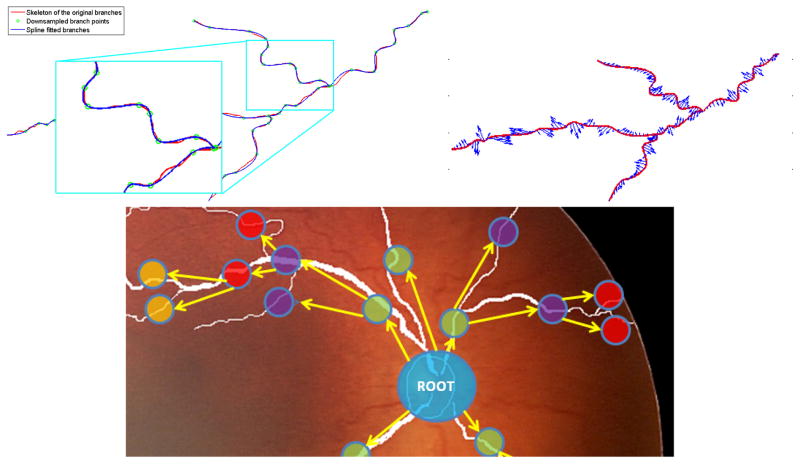
Spline fitting is followed by extraction of the curve-based features that are acceleration (Acc), tortuosity index (TI) and diameter. Acceleration and tortuosity are extracted in a cumulative manner beginning from the initial point of the branch. The diameter is calculated at each sampled point instantaneously by counting the number of white pixels in the direction perpendicular to the curve. Figure 1 displays the spline fitting and the extracted acceleration features from an image in our dataset. Note that the unit for both acceleration and diameter is based on optic disc diameter rather than pixels.

Fig. 1.

Spline fitting (top left) and extracted acceleration vectors with blue arrows on red spline points (top right) and tree representation of an image from the dataset (bottom)

Assuming the optic disc center as the root node, we have created a tree structure treating each branch as a node. Figure 1 shows the tree structure of an image from our dataset. For each node of the tree, we have extracted distance to the disc center (DDC) (i.e. the Euclidean distance between starting point of the branch and the optic disc center ¹). This feature gives idea how far branching occurs. The other tree-based feature is main branch leaf node factor (MBLF), that is the number of leaf nodes per main branch. For a diseased image, MBLF will be high since there will be more bifurcation through the end of the branch.

All features are extracted from arteries and veins separately. For each feature we have computed the two smallest and two largest values, mean, second central moment (CM2) and third central moment (CM3) except MBLF. For MBLF we have computed minimum, maximum, mean, second central moment and third central moment. We have 66 features in total.

2.2. Relationship Between Observers

For each observer pair, we compute the MI based on their decision on the images. Assume the decisions of two observers are X and Y respectively. Then the mutual information between them is:

$$I(X;Y)=\sum _{y\in Y}\sum _{x\in X}p(x,y)log\left(\frac{p(x,y)}{p(x)p(y)}\right)$$ (1)

Since I(X; Y ) = H(X) – H(X|Y ) where H(·) and H(·|·) are entropy and conditional entropy, we create a distance metric between samples, by normalizing mutual information with entropy, and subtracting it from 1,

$$D(X;Y)=1-\frac{I(X;Y)}{H(X)}$$ (2)

2.3. Relationship between Observers and Features

We can compute the mutual information between features and labelers by exploiting Kernel Density Estimation. Assume we have N samples with d dimensional features, f_i ∈ ℝ^d i = {1, 2, … N}. Using a Gaussian kernel, probability density function p(f) is

$$p(\mathbf{f})=\sum _{i=1}^N{G}_{{\mathbf{\sum }}_i}(\mathbf{f}-{\mathbf{f}}_i)$$ (3)

where Σ_i is the variable kernel covariance of the Gaussian kernel $G_{{\mathbf{\sum }}_i}({\mathbf{p}}_{\mathbf{i}})={(2\pi )}^{-d/2}{\mid {\mathbf{\sum }}_i\mid }^{-1/2}{e}^{-\frac{1}{2}{\mathbf{f}}_i^T{{\mathbf{\sum }}_i}^{-1}{\mathbf{f}}_i}$ for the sample i. The estimate of entropy is computed as follows

$$H(F)=\frac{1}{N}\sum _{i=1}^{N}logp({\mathbf{f}}_i)$$ (4)

where F represents the random variable for features. Then MI between feature F and class labels C is computed as I(F ; C) = H(F ) – H(F |C). Note that probability of feature given class will be

$$p(\mathbf{f}\mid c_k)=\sum _{i\in C_k}{G}_{{\mathbf{\sum }}_i}(\mathbf{f}-{\mathbf{f}}_i)$$ (5)

where C_k is the set of indices for the samples from class c_k.

In order to rank features depending on their consistency with the labels, we can compute the MI between each feature and the class labels. The features which provides more information with the labels can be seen as the important features for the observer. However, this approach will not take into account the joint mutual information between multiple features and the class labels. So, as an alternative, we can also select the most important features for a labeler in a recursive manner. With this approach, we pick one feature at a time, which gives the most MI with the labels, when combined with the already selected features. The details of the recursive selection technique can be seen on Algorithm 1.

Algorithm 1.

Algorithm to select best m features given d dimensional features F and class labels C. F^U represents the random variable for features, when only the feature indices listed in U are used. MI(F, C) is the mutual information between F and C. The resulting m feature indices are listed in S.

1:	S ← {}
2:	U ← {1, 2, … d}
3:	while ||S|| < m do
4:	$k\leftarrow \underset{j\in U}{\mathit{argmax}}MI(F^{S\cup \{j\}},C)$
5:	S ← S ∪ {k}
6:	U ← U \ {k}
7:	end while

3. EXPERIMENTS AND RESULTS

Our dataset consists of 34 retinal images diagnosed by 22 observers. Each participant provided one of four mutually exclusive classes of decisions; plus (i.e. plus disease), pre-plus, neither and cannot determine. For data analysis, “cannot determine” decisions were excluded. The veins and arteries are manually segmented by an expert.

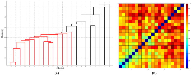
In order to see the relationship between labelers, pairwise distances are computed as stated in equation (2). Then, with single link approach we obtained the dendrogram in Figure 2(a) where we have applied a 0.5 cutoff value. As seen from the figure, a group of observers (red partition) decide consistent to each other, while others are different than the group. Notice that based on different cutoff thresholds, we still end up having one main cluster and the remaining observers as outliers to the main cluster. The distance matrix of labelers is displayed on Figure 2(b), where the order of observers is the same as the order shown in the dendrogram. Hence the observers in the main cluster are shown at the bottom left corner of the distance map. Please also note that defining a ground truth for the images is very difficult although we can find a group of observers with consistent labels.

Fig. 2.

(a)Single link hierarchical clustering with a cutoff value of 0.5 (b) distance map between labelers

We have also computed the MI between labelers and features. Figure 3 shows the colormap, where the labelers in the main cluster are displayed in the first 14 bottom rows. For observer 3, there was only one sample in one of the classes, which prevented us to compute the conditional entropy. Hence we ignored that observer for further analysis. Note that observer 3 is not in the main cluster based on our previous analysis. The features which give the highest MI with at least one observer are, mean tortuosity of veins (for 17 observer), mean acceleration of veins (for 1 observer), mean tortuosity of arteries (for 1 observer), CM2 of tortuosity in arteries (for 1 observer), mean diameter in arteries (for 1 observer).

Fig. 3.

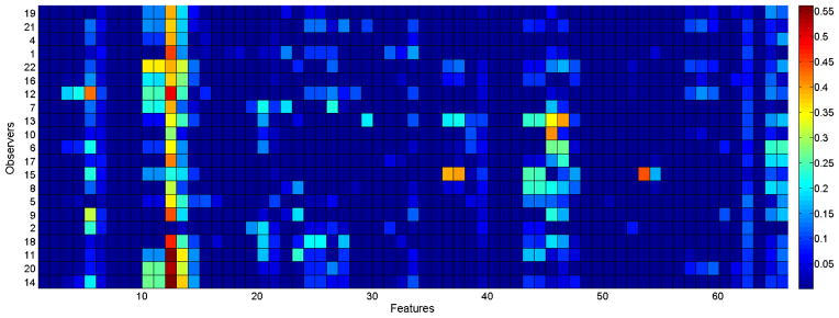
MI between observers and features

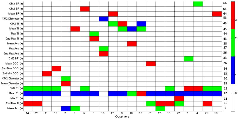
As seen from Figure 3, most of the observers are interested in features 12 and 13, which correspond to mean and CM2 of venular tortuosity. Another bright column is the last column that shows the CM2 and CM3 of the MBLF in arteries. Different than the others, the observers in the main cluster are interested in features 45 and 46, that are mean and CM2 of arteriolar tortuosity. For a better visualization, top three features giving the maximum MI per observer is displayed in Figure 4. The colors represent the rank of the feature for the corresponding observer where white cells indicate that the feature is not among top three.

Fig. 4.

Top 3 features for each observer based on sorting MI values. Feature indexes are displayed at the right side.

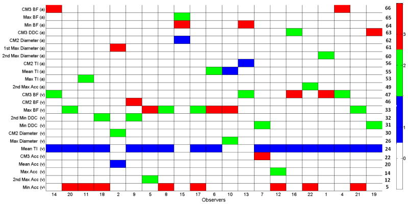
For each observer, we have also determined the most important features by our recursive selection scheme. Figure 5 displays three selected feature per labeler. Even though some features such as minimum acceleration or minimum DDC are not distinctive enough, they are selected with this approach. Because, the technique involves joint MI of a set of features rather than MI of each feature independently.

Fig. 5.

Three best features for each observer using recursive selection scheme. Feature indexes are displayed at the right side.

4. CONCLUSION AND DISCUSSION

In this paper, we propose a method to analyze observer and feature relationships for the diagnoses of ROP disease. A large set of features are extracted in two categories; curve-based and tree-based features. The experiments are carried out on 34 retinal images that are diagnosed by 22 experts. The results show that there is consistency between the decisions of a large group of observers. Based on the analysis, a list of features that are correlated with the expert decisions are reported. In the future, we plan to create an interactive automated classification system with feature and observer analysis modules on a larger dataset of images and observers.

References

- 1.Early Treatment For ROP Cooperative Group. Revised indications for the treatment of retinopathy of prematurity; results of the early treatment for retinopathy of prematurity randomized trial. Arch Ophthalmol. 2003;121:1684–1694. doi: 10.1001/archopht.121.12.1684. [DOI] [PubMed] [Google Scholar]
- 2.Gilbert C, Foster A. Childhood blindness in the context of VISION 2020–the right to sight. Bull World Health Organ. 2001;79(3):227–232. [PMC free article] [PubMed] [Google Scholar]
- 3.Gilbert C, Fielder A, Gordillo L, et al. Characteristics of infants with severe retinopathy of prematurity in countries with low, moderate, and high levels of development: Implications for screening programs. Pediatrics. 2003;115:518–525. doi: 10.1542/peds.2004-1180. [DOI] [PubMed] [Google Scholar]
- 4.Kemper AR, Wallace DK. Neonatologists practices and experiences in arranging retinopathy of prematurity screening services. Pediatrics. 2007;120:527–531. doi: 10.1542/peds.2007-0378. [DOI] [PMC free article] [PubMed] [Google Scholar]
- 5.The Committee for the Classification of Retinopathy of Prematurity. An international classification of retinopathy of prematurity. Arch Ophthalmol. 1984;102:1130–1134. doi: 10.1001/archopht.1984.01040030908011. [DOI] [PubMed] [Google Scholar]
- 6.The Committee for the Classification of Retinopathy of Prematurity. The international classification of retinopathy of prematurity revisited. Arch Ophthalmol. 2005;123:991–999. doi: 10.1001/archopht.123.7.991. [DOI] [PubMed] [Google Scholar]
- 7.Chiang MF, Jiang L, Gelman R, Du YE. Inter expert agreement of plus disease diagnosis in retinopathy of prematurity. Arch Ophthalmol. 2007;125:875–880. doi: 10.1001/archopht.125.7.875. [DOI] [PubMed] [Google Scholar]
- 8.Wallace DK, Quinn GE, Freedman SF, Chiang MF. Agreement among pediatric ophthalmologists in diagnosing plus and pre-plus disease in retinopathy of prematurity. J AAPOS. 2008;12:352–356. doi: 10.1016/j.jaapos.2007.11.022. [DOI] [PMC free article] [PubMed] [Google Scholar]
- 9.Wallace David K, Jomier Julien, Aylward Steven R, Landers Maurice B., III Computer-automated quantification of plus disease in retinopathy of prematurity. Journal of American Association for Pediatric Ophthalmology and Strabismus. 2003;7(2):126– 130. doi: 10.1016/mpa.2003.S1091853102000150. [DOI] [PubMed] [Google Scholar]
- 10.Gelman R, Martinez-Perez ME, Vanderveen DK, Moskowitz A, Fulton AB. Diagnosis of plus disease in retinopathy of prematurity using retinal image multiscale analysis. Investigative ophthalmology & visual science. 2005;46(12):4734–4738. doi: 10.1167/iovs.05-0646. [DOI] [PMC free article] [PubMed] [Google Scholar]
- 11.Wilson CM, Cocker KD, Moseley MJ, Paterson C, Clay ST, Schulenburg WE, Mills MD, Ells AL, Parker KH, Quinn GE, et al. Computerized analysis of retinal vessel width and tortuosity in premature infants. Investigative ophthalmology & visual science. 2008;49(8):3577–3585. doi: 10.1167/iovs.07-1353. [DOI] [PubMed] [Google Scholar]
- 12.Shah DN, Wilson CM, Ying G, Karp KA, Fielder AR, Ng J, Mills MD, Quinn GE. Semiautomated digital image analysis of posterior pole vessels in retinopathy of prematurity. Journal of American Association for Pediatric Ophthalmology and Strabismus. 2009;13(5):504–506. doi: 10.1016/j.jaapos.2009.06.007. [DOI] [PubMed] [Google Scholar]
- 13.Gelman R, Jiang L, Du YE, Martinez-Perez ME, Flynn JT, Chiang MF. Plus disease in retinopathy of prematurity: pilot study of computer-based and expert diagnosis. Journal of American Association for Pediatric Ophthalmology and Strabismus. 2007;11(6):532–540. doi: 10.1016/j.jaapos.2007.09.005. [DOI] [PMC free article] [PubMed] [Google Scholar]
- 14.Koreen S, Gelman R, Martinez-Perez ME, Jiang L, Berrocal AM, Hess DJ, Flynn JT, Chiang MF. Evaluation of a computer-based system for plus disease diagnosis in retinopathy of prematurity. Ophthalmology. 2007;114(12):e59–e67. doi: 10.1016/j.ophtha.2007.10.006. [DOI] [PubMed] [Google Scholar]
- 15.Wallace DK, Freedman SF, Zhao Z, Jung SH. Accuracy of roptool vs individual examiners in assessing retinal vascular tortuosity. Archives of ophthalmology. 2007;125(11):1523. doi: 10.1001/archopht.125.11.1523. [DOI] [PubMed] [Google Scholar]
- 16.Van Uitert R, Bitter I. Subvoxel precise skeletons of volumetric data based on fast marching methods. Medical physics. 2007;34:627. doi: 10.1118/1.2409238. [DOI] [PubMed] [Google Scholar]
- 17.Douglas DH, Peucker TK. Algorithms for the reduction of the number of points required to represent a digitized line or its caricature. Canadian Cartographer. 1973;10:112–122. [Google Scholar]