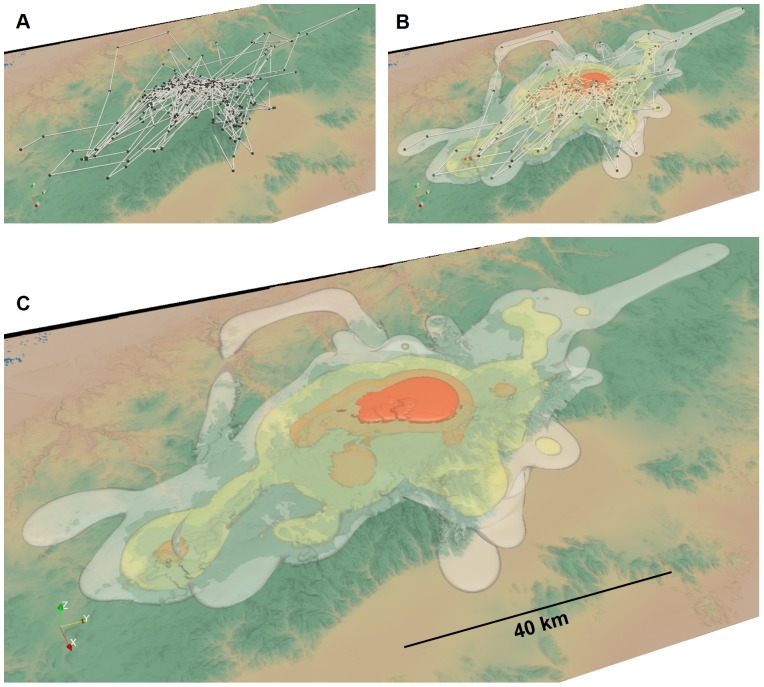
Figure 3. An illustration of the steps in generating a 3D MKDE for a California condor.
The 3D MKDE is constructed from observed 3D locations and a digital elevation model that sets the lower bound on the MKDE. The expected location (gray points) at each unobserved time is determined by linear interpolation (white lines) between the observations (A). The 3D MKDE is then constructed by integrating a trivariate normal distribution, possibly constrained above or below in the z-dimension, over time along the interpolated movement path (B). The variance of the kernel increases as it moves further from the times of the observed locations. The contours of the final 3D MKDE is shown in C. In B and C, the 99%, 95%, and 50% 3D MKDE volumes are shown in transparent white, orange, and red, respectively.

