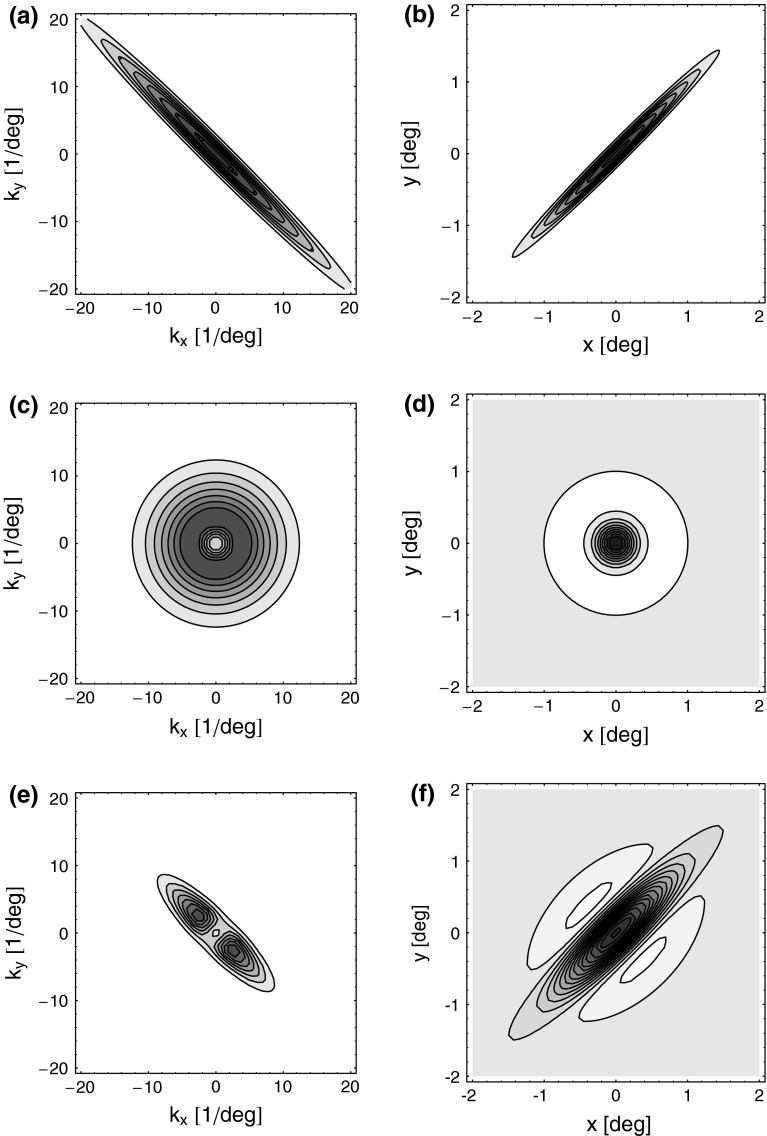
Fig. 2.
Contour plots illustrating spatial part of loop kernel (a, b) and model impulse-response functions (c, d) for relay-cell (DOG model) and impulse-response “input” to cortical cell (e, f). Functions are shown in Fourier-space in the left column (a, c, e) and in real space in the right column (b, d, f). (a) Fourier-space loop kernel for cortical feedback loop modeled as a Gaussian ellipse,  in Eq. 20 (θn = π/4, σn = 0.1 deg, σl = 1.4 deg,
  ). (b)
  Eq. 19 corresponding to
  . (c) Fourier-space relay-cell DOG model
  from Eq. 7 (A
1 = 1, a
1 = 0.25 deg, A
2 = 0.85, and a
2 = 0.83 deg). (d) f
DOG(r) (from Eq. 6) corresponding to
  . (e) Fourier-transformed input to cortical cell
  . The spatial parameters for the feedforward coupling kernel
  are chosen a factor
  smaller than for the loop kernel
  , i.e., σn = 0.07 deg, σl = 0.99 deg, while
  . With the same spatial parameters for a similarly modeled feedback coupling kernel
  , one would get the loop kernel
  in panel (a). (f)
 found by an inverse Fourier-transform of
  . In panels (a), (b), (c) and (e) white corresponds to the zero level; in panels (d) and (f) white corresponds to a negative value to illustrate the negative lobes of the LGN (DOG) receptive fields and input to cortical cells (subthreshold receptive fields)

