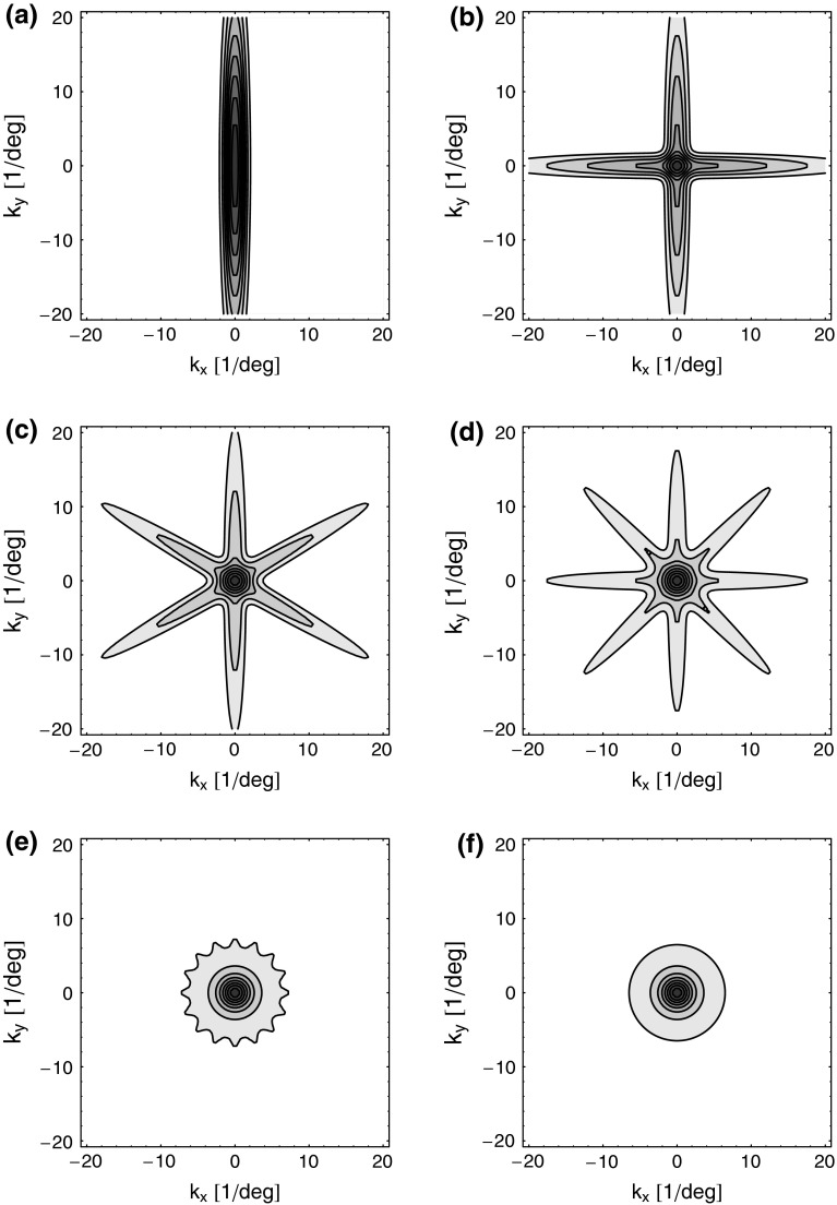
Fig. 3.

Example contour plots of the summed spatial loop kernel including several excitatory cortical feedback loops, Eq. 22, for different numbers of cortical populations N. The Gaussian width parameters are chosen as in Fig. 2, i.e., σ_n = 0.1 deg, σ_l = 1.4 deg. Here we use which assures the same overall coupling strength (summed over all k-space) in the set of examples. (a) N = 1, (b) N = 2, (c) N = 3, (d) N = 4, (e) N = 8, (f) , Eq. 24