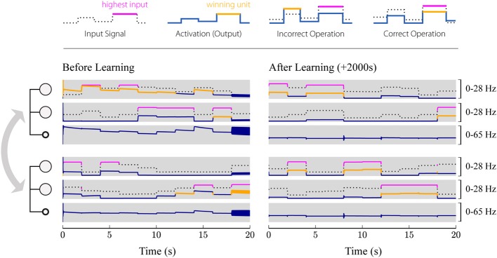
Figure 7.

Simulated evolution of the plastic network. 1000 input patterns were applied for 2 s each. Two local subsystems, consisting of two excitatory units and one inhibitory unit each, are coupled via all-to-all excitatory connections, while inhibitory feedback is provided only locally. The first three rows show the populations of the first group, where the first two rows correspond to the two excitatory populations, and the third row shows the activation of the inhibitory population. The last three rows show the activations of the second group. The left panel shows the first 20 s after initialization (before learning), while the right panel shows the network activity during the last 20 s (after learning). Solid blue and orange lines correspond to the firing rate of the respective population, whereby the highlighted segments (orange) mark the winner among the four excitatory populations. The input given to the individual units is plotted as a dotted black or solid magenta line, where the highlighted segments (magenta) correspond to the strongest signal among the four. Thus, the network operates correctly if magenta and orange lines are aligned (the one population that receives the strongest input wins the competition), while misaligned lines (the population receiving the strongest input does not win the competition) indicate incorrect operation. Initially, the network frequently selects the wrong winning unit and even starts oscillating for some input patterns (around 18 s). After training (right), the network converges to a stable state with only the winning unit active for different input patterns.