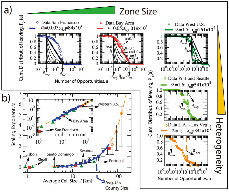
Figure 3. Interpretation of the parameter α.

(a) Effects of the scale on the P_>(a) distribution, showing as symbols the results from census data of San Francisco, the Bay area and the Western U.S. The black solid lines are evaluations of Eq. 13 for different values of α, and the dashed line is the expected α value using Eq. 14. The analytical predictions work for the Bay area and Western U.S. From top to bottom we see the P_>(a) distribution for three regions with similar sizes. Given a fixed scale, the α value is influenced by the heterogeneity of the distribution of opportunities. The more heterogeneous the region is, the larger the difference between a_avg and a_min, as is shown in Las Vegas-L.A. region. In these cases the prediction of α (Eq. 13) will not resemble their calibrated values and thus calibration is needed. (b) For each zone scale l, 200 regions with random centers are selected within west U.S. In each case the corresponding α value is calibrated with census trip data. The functional relationship between α and l is . The error bar shows the 20 and 80 percentile α value for each scale. The inset shows the same plot in logarithmic scale. Marked as solid blue circles is the scale range that α values can be predicted without data calibration. The calibrated results with trip data for U.S. regions are marked as red squares, while the examples from other countries are marked as green triangles. They all follow the functional approximation.