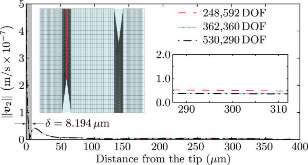
Fig. 4.

Plot of the magnitude of the second-order velocity vs. position along a line parallel to the y axis and emanating from the tip of a sharp edge (red line in left inset). The different curves correspond to different levels of adaptive refinement. The inset on the left shows the initial mesh used for the calculations. The right inset shows a zoomed-in portion of the plot outside the Stokes boundary layer of thickness δ. The units on the vertical axis of the right inset are the same as those on the overall plot.