
Fig. 4.
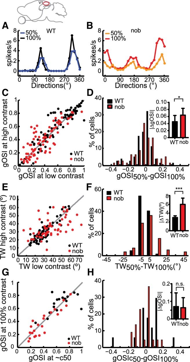
Slight disruption of contrast invariance of orientation tuning in nob V1. A and B: examples of orientation tuning curves at low (50%) and high (100%) contrasts in WT (A) and nob (B) mice. C: scatter plot of gOSI at low (50 or 60%) vs. high (100%) contrast. Black dots: WT, n = 81; red dots: nob, n = 80 cells. Gray line indicates unity. D: distribution of differences in gOSI at the 2 contrasts. Inset: average of absolute differences. E: scatter plot of tuning width (half height at half maximum) at low (50 or 60%) vs. high (100%) contrast. WT, n = 67; nob, n = 58 cells. F: distribution of differences in tuning widths at the 2 contrasts. Inset: average of absolute differences. G and H: gOSI near the half-saturation contrast (c50) of each cell is compared against its gOSI at 100% contrast. WT, n = 20; nob, n = 34 cells. H: average of absolute differences in gOSI. All bars indicate means + SE. *P < 0.05 and ***P < 0.001.