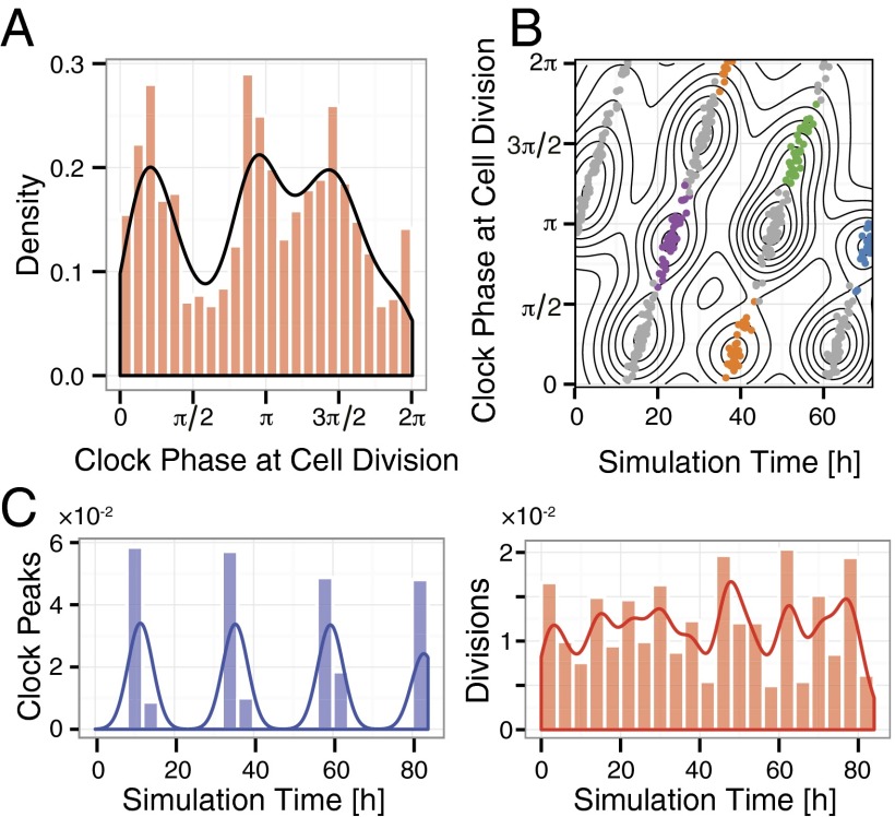
Fig. 6.

Modeling stochastic 3:2 coupling. (A) A plot similar to Fig. 4D, Left but for modeled stochastic 3:2 coupling. In this case, we observe three peaks of cell division phases, corresponding to the three crossings of the attracting trajectory with the curve corresponding to cell division (the labeled horizontal line in Fig. 5C). (B) Clustering of the modeled cell divisions as in Fig. 4 A and B. There are essentially two sets of clusters, each group coming from (i.e., containing descendant cells of) the initial two clusters at the left. In the experiments only one of these sets is populated, presumably because of the way the synchronization works and the existence of other states (e.g., 1:1) after perturbation. This set is colored and the other is in gray. (C) We also see that although population-level synchronization of the clock is clear (Left), synchronization of cell cycle is not visible (Right), because the cell divisions cluster too closely in time and the projection onto the time axis is without clear peaks. We can still see the clusters of divisions in B when separating them out both in clock phase and time.