Figure 4.
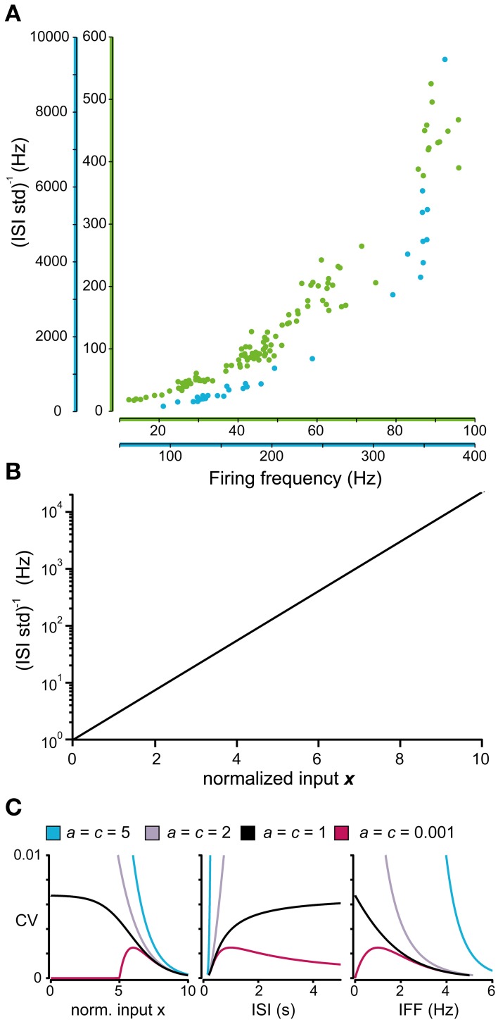
Relationship between firing level and spike firing variability. (A) Relationship between the firing frequency and the inverse of the standard deviation of the ISIs for two sample spinal interneurons. Note that the axes of the firing frequency for the two neurons differ substantially. (B) Model prediction of the relationship between the normalized input and the logarithmic value of the inverse of the standard deviation of the ISI distribution. (C) Predicted coefficient of variation (CV) of the complete model in Equation (6) where the parameters a and c are varied as in Figure 3. (C; left) Relationship between the normalized input and the CV. Note that the CV only reaches a stable value above 0 as the input approaches −∞ (corresponding to a substantial hyperpolarization) if c = 1. Otherwise it either diverges as c > 1 or approach 0 as c < 1. (C; middle, right) For comparison with previous results, the CV in relation to the average length of the ISIs (middle) (Softky and Koch, 1993) and the CV in relation to the instantaneous firing frequency (right) (Rauch et al., 2003) is also included in the figure.

