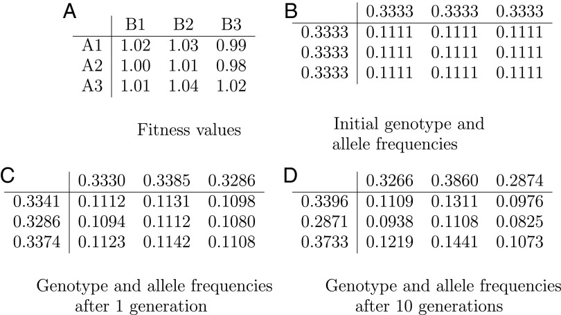
Fig. 1.

Equations of population genetics formulated in the 1930s constitute the standard mathematical way of understanding evolution of a species by tracking the frequencies of various genotypes in a large population. In the simple example shown here, a haploid organism with two genetic loci A and B has three alleles in each of its two loci named A1, A2, A3 and B1, B2, B3 for a total of nine genotypes. In A we show the fitness of each genotype, that is, its expected number of offspring. The fitness numbers shown in A are all close to each other, reflecting weak selection, where the individual alleles’ contributions to fitness are typically minuscule. Initially, each genotype occurs in the population with some frequency; in this particular example these numbers are initially equal (B); naturally, their sum over all nine genotypes is 1 (frequencies are truncated to the fourth decimal digit). C shows how the genotype frequencies evolve in the next generation: each individual of a given genotype produces a number of offspring that is proportional to its fitness shown in A, and the resulting offspring inherits the alleles of its parents with equal probability (because we are assuming, crucially, sexual reproduction). The genotype frequencies in the next generation are shown in C, calculated through the standard recurrence equations of population genetics. We also show in the margins of the table the allele frequencies, obtained by adding the genotype frequencies along the corresponding row or column. Ten generations later, the frequencies are as shown in D.