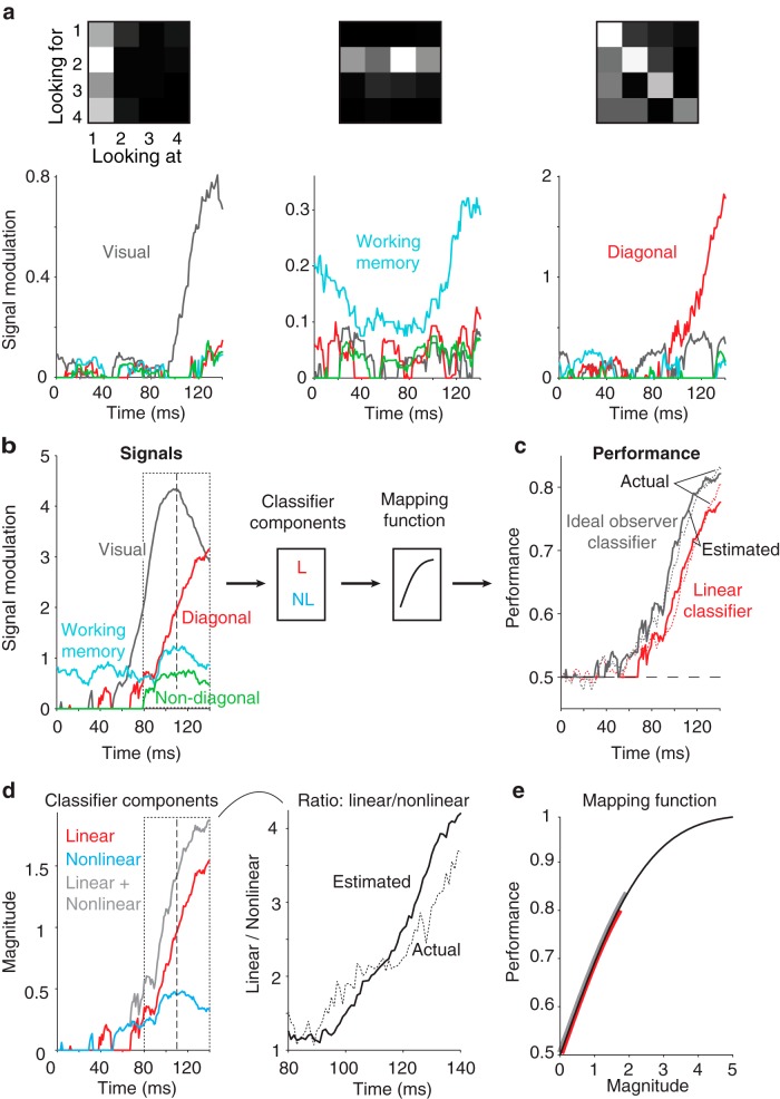
Figure 4.

Single-neuron decomposition of population untangling dynamics in PRH. To determine the relationship between single-neuron response properties and population performance measures, we applied a method to parse each neuron's responses into intuitive signal modulation components, including firing rate modulations that could be attributed to: visual—changes in the visual image; working memory—changes in the identity of the target; diagonal—whether a condition was a target match or distractor; non-diagonal—other cognitive modulations (see Materials and Methods, Eqs. 7,8). We note that the method estimates and corrects for noise to ensure that trial-by-trial variability is not confused with signal. a, Plotted is the strength of each type of modulation (Eq. 8) as a function of time relative to stimulus onset, for three example neurons whose responses are dominated by one type of modulation. Also shown are the firing rate response matrices for each neuron, with spike counts averaged within the same window (0–140 ms after stimulus onset), each rescaled from the minimum (black) to maximum (white) firing rate. b, Left, The same plots depicted in a, but summed over all neurons in the PRH population. Right, The relationship between these signal modulation magnitudes and performances for the ideal observer and linear classifier can be described as a classifier component computed from the underlying signals followed by a mapping function that transforms the component values into performances. The classifier component for the linear classifier was computed from the diagonal signal alone. The classifier component for the ideal observer was computed by summing the linear classifier component signal with a second nonlinear classifier component that nonlinearly combined the visual and other cognitive signals (working memory and non-diagonal cognitive; see Materials and Methods, Eqs. 13–15). The same mapping function was used for both classifier predictions. c, Time courses for the actual (dotted, replotted from Fig. 3b, left) and estimated (solid) classifier performance values. d, Time courses of the linear, nonlinear, and summed classifier component signals. e, Time course for the actual (dotted, replotted from Fig. 3d) and estimated (solid, based on the data on the left) ratios of chance-corrected linear and nonlinear classifier components with the same conventions as Figure 3d, right. f, The mapping function used to convert classifier component magnitudes into performance predictions. The red and gray lines indicate the range of values used to estimate the linear and ideal observer, respectively. In b and d, the dotted box from 80 to 140 ms and the dashed line at 110 ms are provided as visual benchmarks.