Fig. 3.

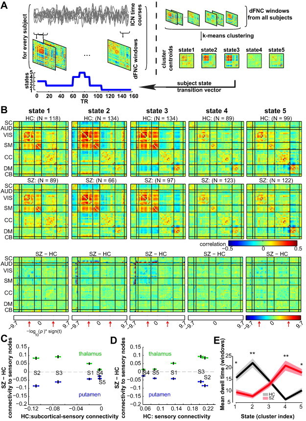
A) Schematic depicting the computation of the state transition vector for each subject. First, dFNC matrices are computed on windowed portions of the ICN time courses. Then, dFNC matrices from all subjects are clustered using the k-means algorithm, yielding cluster centroids and cluster membership assignment for all windows. When viewed in time, the window membership represents the state transition vector. B) The medians of cluster centroids by state for HC (top) and SZ (middle) along with the count of subjects that had at least one window in each state are shown. The bottom row shows the results of two sample t-test results performed across subject median dFNC maps by state, with the FDR threshold (q < 0.05) indicated by red arrows. (C–D) Illustration of the dependence of group differences on connectivity states/patterns. In (C), the group difference (SZ–HC) in thalamic-sensory connectivity, and putamen–sensory connectivity are plotted as a function of subcortical-sensory antagonism (average of cells within subcortical to sensory nodes) found in each state averaged over HC. In (D), the same group differences are displayed as a function of sensory connectivity. The error bars in (C–D) are obtained using bootstrap resampling. E) The mean ± standard error of dwell times by state for HC (black) and SZ (red). Asterisks indicate p < 0.05 (FDR corrected) and double asterisks indicate p < 0.001 (FDR corrected), as obtained via two-sample t-tests.