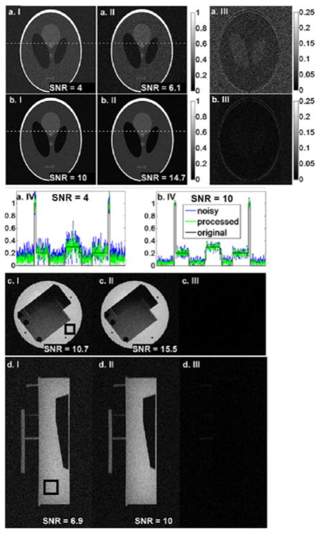
Fig. 2.

Simulated Shepp–Logan phantom (rows a and b) and MRI phantom magnitude images (rows c and d) are shown. Original noisy images (column I), processed images (column II), and the residuals (column III) are displayed. Pro-files of the image along the dotted lines in (a.I), (a.II) and (b.I), (b.II) are plotted in (a.IV) and (b.IV), respectively. SNR improvement of ~40% is observed. Noise level is calculated from the background and signal intensity is calculated by averaging the pixels in a uniform region as indicated by the square box.