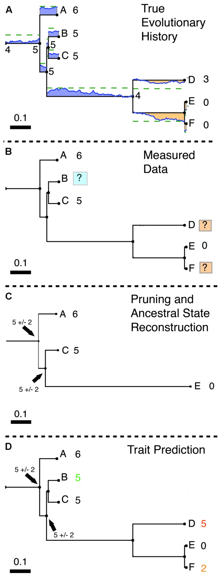
FIGURE 1.

Hidden State Prediction (HSP). (A) Evolution of a simulated trait following a Brownian motion model. For example, the copy number of a gene family in each of several microbial genomes can be mapped onto a phylogenetic tree and represented as a continuous trait. (The same method could be used on any continuous evolutionary character.) Here, a trait starting with a value of 4 evolves by a Brownian motion process within a group of organisms A–F. Blue values above each edge of the phylogeny indicate regions of the phylogeny where the trait takes on a value greater than 4 (gain with respect to the ancestor of A–F). Orange values below the edges indicate trait values lower than 4 (loss relative to the ancestor). Numbers by the tips of the tree show the final value of the trait rounded to the nearest integer, as when the trait is taken to represent the copy number for a particular gene. (B) Observed Data. In general only a portion of all modern organisms are sampled. In this example trait values have been measured for tips A, C, and F but are unknown for tips B, D, and E.The tips with unknown trait values differ in their proximity to characterized relatives. Tip D is only distantly related to tips with known values. Note that tip B is closely related to tips A and C for which trait values are known. Thus for B the closest known tip is within 0.12 units of branch length, whereas for D the closest tip is 0.63 units of branch length away. The task of HSP is to estimate trait values for B, D, and F from the values for A, C, and E. Examples of tips for which trait prediction will be more or less accurate are shaded with blue or orange boxes, respectively. This task will be simplest in cases like B in which several close relatives have been assayed and hardest in cases like D where long branches separate unknown tips from known references. (C) Ancestral State Reconstruction (ASR). The unknown tips are dropped from the tree (most phylogeny programs cannot handle missing character values) and ancestral character values are calculated for the remaining internal nodes. (An alternative method for discussed in the text is to repeatedly reroot the tree at each node of interest (here B,D,F) and perform standard ASR (Garland and Ives, 2000). (D) Prediction of character values. If prediction via tree rerooting is not used, the inferred ancestral states and evolutionary model must be extended to the tips using another method. For example, the predictive functional profiling software package PICRUSt (which predicts metagenomic counts from marker gene data; see main text) uses exponential weighting by branch length to extend reconstructed states to the tips, and inflates the variance of the reconstructed ancestral state to account for evolution between the ancestor and the tip of interest (Langille et al., 2013). In this example, Tip B, with close references A and C is assigned correctly. Tips D and F, where such references are either missing (tip D) or available only in a sister group (but not a closely related outgroup; F) are assigned less accurately (both off by two copies). However, D is correctly inferred to have more copies than F. Note that this example is intended to illustrate compactly the algorithm and some examples of success or failure, and should not be taken to represent the average accuracy of these methods, which have been studied in some depth (see Factors Influencing the Accuracy of Hidden State Prediction Algorithms for a summary of major findings).