Optimal Denoising in Redundant Representations

Abstract

Image denoising methods are often designed to minimize mean-squared error (MSE) within the subbands of a multi-scale decomposition. However, most high-quality denoising results have been obtained with overcomplete representations, for which minimization of MSE in the subband domain does not guarantee optimal MSE performance in the image domain. We prove that, despite this suboptimality, the expected image-domain MSE resulting from applying estimators to subbands that are made redundant through spatial replication of basis functions (e.g., cycle spinning) is always less than or equal to that resulting from applying the same estimators to the original nonredundant representation. In addition, we show that it is possible to further exploit overcompleteness by jointly optimizing the subband estimators for image-domain MSE. We develop an extended version of Stein’s unbiased risk estimate (SURE) that allows us to perform this optimization adaptively, for each observed noisy image. We demonstrate this methodology using a new class of estimator formed from linear combinations of localized “bump” functions that are applied either point-wise or on local neighborhoods of subband coefficients. We show through simulations that the performance of these estimators applied to overcomplete subbands and optimized for image-domain MSE is substantially better than that obtained when they are optimized within each subband. This performance is, in turn, substantially better than that obtained when they are optimized for use on a nonredundant representation.

I. Introduction

Image denoising has undergone dramatic improvement over the past decade, due to both the development of linear decompositions that simplify the characteristics of the signal, and to new estimators that are optimized for those characteristics. A standard methodology proceeds by linearly transforming the image, operating on the transform coefficients with nonlinear estimation functions, and then inverting the linear transform to obtain the denoised image. Estimation functions generally take the form of “shrinkage” operators that are applied independently to each transform coefficient (e.g., [1]–[8]), or are applied to neighborhoods of coefficients at adjacent spatial positions and/or from other subbands (e.g., [9]–[12]).

The choice of estimation function is an essential part of the denoising problem. From a statistical perspective, one may use a prior probability model for the transform coefficients (either assumed, or fit to a set of clean training images), and then use this to derive a Bayes-optimal estimator. Alternatively, one may directly assume a parametric form for the estimation function, and select parameters by optimizing performance on a training set containing pairs of clean images and their noisy counterparts (e.g., [13]). As described, these methodologies require explicit information about clean images, either through samples or knowledge of the prior distribution, both of which will typically reflect the statistics of heterogeneous ensembles of images. However, there are ways of adaptively optimizing the parameters of the density model for the particular image being de-noised. For example, an “empirical Bayes” estimator may be derived from a prior density whose parameters are chosen to best account for the observed noisy image (typically, by maximizing likelihood) [3]. A parametric estimator may also be adaptively optimized by minimizing Stein’s unbiased risk estimate (SURE) [14], which provides an approximation of the mean squared error (MSE) as a function of the observed noisy data. Assuming there is enough data to capture the statistics of a given image, adaptive methods will always perform better than those optimized for a heterogeneous ensemble of images.

Although it is less well understood, the choice of linear transform also has an impact on the quality of denoising results. Multiscale decompositions are a typical choice, and both empirical Bayes methods [3], [5], [8], and SURE adaptive methods have been used to optimize scalar [31], [16]–[18], [22] and joint [15] estimators for application to subbands of multiscale decompositions. Empirical evidence indicates that redundant (overcomplete) multiscale representations are more effective than orthonormal representations [19], [20]. This fact is somewhat mysterious, since the estimators are generally optimized for MSE within individual subbands, which (for a redundant basis) is not the same as the MSE in the image domain. Recent work provides an interesting explanation for this phenomenon by interpreting shrinkage in overcomplete representations as the first iteration of a Basis Pursuit denoising algorithm [21].

In this paper, we prove that application of denoising functions to subbands made overcomplete through cycle spinning or elimination of decimation is guaranteed to be no worse in MSE (and is in practice significantly better) than applying the same functions in an orthonormal basis. This method of denoising, however, does not take full advantage of the redundancy, and further improvements may be obtained by jointly choosing subband denoising functions that optimize MSE in the image domain. We provide a method for this image-domain optimization by extending SURE to approximate the image-domain MSE that results from applying estimation functions to coefficients of a redundant basis. We develop a family of parametric estimators based on a superposition of localized “bump” functions, and demonstrate through simulations that optimizing the image-domain SURE of these estimators applied within undecimated wavelet subbands leads to significant performance improvements over optimizing the subband-domain SURE of the same estimators. A preliminary version of this work has been presented in [22].

II. Redundancy Improves Performance

Given a noisy image Y, we wish to compute an estimate of the original (clean) image X̂(Y) = f(Y), where the estimator f is selected from a family to minimize the MSE

$$f_{\text{opt}}=arg\underset{f\in \mathcal{F}}{min}E\{{\mid X-f(Y)\mid }^2\}$$

and E{ } indicates the expected value. We may consider X to be fixed but unknown (the so-called “frequentist” perspective), with the expectation taken over Y conditioned on X. Alternatively, we may consider X to be a sample drawn from some prior probability distribution p_x(X) (the “Bayesian” perspective). In this case, the expectation is taken jointly over X and Y, or (equivalently) over Y conditioned on X, and then over X.

A common practice in image denoising is to use estimators that act on a linearly transformed version of the corrupted image, U = WY. Here, W can be a complete or overcomplete linear transformation (an m by n matrix, m ≥ n, where n is the dimension of image space), that has a left inverse W^† such that W^†W = Id. In this section, we assume that the transform is a tight frame, for which W^† = W^T. This includes orthogonal, cycle-spun and undecimated wavelet transforms, as well as other overcomplete decompositions such as the steerable pyramid [23], curvelets [24], or complex dual-tree wavelets [25].

In this situation, the estimate is computed by transforming the original signal, applying an estimator f_u in the transform domain, and then inverse transforming with W^T

$$f(Y)=W^T{f}_u(WY).$$

The MSE incurred in using this estimator is thus

$$E\{{\mid X-W^T{f}_u(WY)\mid }^2\}=E\{{\mid W^T(V-f_u(U))\mid }^2\}$$ (1)

where V = WX, the transform of the clean image. Note that in the case when W is orthogonal, the transform preserves vector lengths (as does W^T), and the MSE reduces to E{|(V^o − f_u(U^o))|²}, where the superscripts on U, V are a reminder that the coefficients were obtained from an orthogonal transform. In the next sections, we explain why and under what conditions the performance of a denoising function on an orthonormal wavelet basis can be improved by adding redundancy to the transform through cycle spinning or elimination of decimation. For didactic purposes, we will consider cycle spinning.

A. Scalar Estimators

Consider an estimator f_u composed of scalar functions f_i that operate pointwise on the transform coefficients. Typically, the transform coefficients are partitioned into subbands { ; k = 1, 2, … K}, corresponding to shifted versions of the same basis function, all of which can be assumed to have the same marginal statistical properties. In this case, the same estimator will be applied to all coefficients within each subband, and the MSE can be partitioned into a sum of MSEs on each subband. If we assume an orthogonal transform, we can write the MSE as

$$\begin{array}{l}E\{{\mid (V^o-f_u(U^o))\mid }^2\}=E\left\{\sum _k\sum _{i\in {\mathcal{S}}_k}{\mid V_i^o-f_k(U_i^o)\mid }^2\right\}\\ =\sum _k\sum _{i\in {\mathcal{S}}_k}E\left\{{\mid V_i^o-f_k(U_i^o)\mid }^2\right\}.\end{array}$$ (2)

Now consider a cycle-spun decomposition, in which the basis functions of the original orthonormal representation are replicated at N translated positions [19]. Each subband will contain N times as many coefficients as the corresponding subband of the orthonormal representation. In order to form a tight frame, each basis function must be divided by a factor of $\sqrt{N}$, relative to those of the orthonormal representation. Thus, if f_k is the marginal function used to denoise coefficients in the orthonormal wavelet representation, the corresponding function that should be applied in the cycle-spun decomposition is

$$f_k^c(u)=\frac{1}{\sqrt{N}}{f}_k(\sqrt{N}u).$$

In addition to the tight frame assumptions, we also assume that relationship between the noisy and clean coefficients in each band will be the same (up to a factor of $\sqrt{N}$) in the cycle-spun representation as in the orthonormal representation. Specifically, we assume the joint statistics of the rescaled cycle-spun coefficients, ( $\sqrt{N}{U}^c,\sqrt{N}{V}^c$) are the same as those of the orthogonal coefficients, (U^o, V^o). This allows us to rewrite (2), in terms of the cycle-spun coefficients

$$\begin{array}{l}\sum _k\sum _{i\in {\mathcal{S}}_k}E\{V_i^o-f_k{(U_i^o)}^2\}=\sum _k\frac{1}{N}\sum _{i\in {\mathcal{S}}_k}E\left\{\left|\sqrt{N}{V}_i^c-f_k{\left(\sqrt{N}{U}_i^c\right)}^2\right|\right\}\\ =\sum _k\sum _{i\in {\mathcal{S}}_k}E\left\{{\left|V_i^c-\frac{1}{\sqrt{N}}{f}_k\left(\sqrt{N}{U}_i^c\right)\right|}^2\right\}\\ =\sum _k\sum _{i\in {\mathcal{S}}_k}E\left\{{|V_i^c-f_k^c(U_i^c)|}^2\right\}\\ =E\left\{{\mid V^c-f_u^c(U^c)\mid }^2\right\}.\end{array}$$ (3)

Combining (2) and (3), we see that the MSE in the orthonormal case is equal to the total subband-domain MSE in the cycle-spun case.

Now it is straightforward to compare the MSE in the orthonormal case, as given by (2) or (3), to the image-domain MSE incurred with cycle-spun denoising, as specified by (1)

$$\begin{array}{l}E\{{\mid V^o-f_u(U^o)\mid }^2\}=E\left\{V^c-f_u^c(U^c){\mid }^2\right\}\\ \ge E\left\{{\mid W^T(V^c-f_u^c(U))\mid }^2\right\}\end{array}$$

where the inequality holds because W is an overcomplete tight frame, and, thus, W^T is a projection operator. That is, the image-domain MSE for the cycle-spun case is always less than or equal to that for the cycle-spun case. Note that we have assumed nothing regarding the form of the estimators f_k. We also assumed very little about the corruption process—only that it is stationary. The result may be easily extended to undecimated wavelets, in which the number of coefficients in each band will be multiplied by a different factor.

The upshot is that, as long as the joint statistics of pairs of clean and noisy coefficients do not change when going to a redundant basis (as is the case for stationary image and noise statistics), then the performance of any marginal denoising function on the redundant basis is guaranteed to be no worse then the corresponding operations performed on the orthonormal representation. In particular, if we choose an optimal estimator to de-noise each subband of an orthogonal transform, the optimal estimator for the subbands of the redundant basis will be the same (up to rescaling by $\sqrt{N}$), and the performance of the redundant system will generally be better than that of the orthogonal one.

B. Context Estimators

Thus far, we have been discussing scalar estimation functions. However, recent literature has demonstrated that substantial improvements can be achieved with estimators that operate on the surrounding “context” of multiscale coefficients (e.g., [9], [10], [11], [12], [15], [26], [27], [28]). In general, the surrounding neighborhood can include coefficients within the same subband, as well as coefficients in other subbands, and the neighborhoods are generally overlapping (i.e., each coefficient belongs to more than one neighborhood). For our purposes, we handle the overlap of neighborhoods by computing an estimate only for the center coefficient (as in [10]–[12])

$${\widehat{V}}_i({\mathbf{U}}_i)=f_k({\mathbf{U}}_i).$$ (4)

Thus, each coefficient is denoised as a function of its surrounding neighbors. Analogous to the scalar case, we can prove that, for certain neighborhood types, applying a vector denoising function to the subbands of a representation made redundant by spatial replication of orthonormal basis functions leads to improvement in denoising performance over using the original orthonormal basis. In an orthonormal basis, the MSE given by (2) is replaced by

$$E\{{\mid (V^o-f_u(U^o))\mid }^2\}=\sum _k\sum _{i\in {\mathcal{S}}_k}E\left\{{\mid V_i^o-f_k({\mathbf{U}}_i^o)\mid }^2\right\}.$$

We now want to express this error in terms of the neighborhoods of the redundant representation. In order to do so, we must ensure that the neighborhoods in both representations have the same statistics (appropriately scaled). The easiest way to achieve this is to use the same sampling pattern. In a cycle-spun representation, we simply draw adjacent neighbors from within the shifted copies of the original orthonormal decomposition. In an undecimated wavelet, we must choose neighbors of a coefficient on a subsampled lattice, with subsampling factor the same as that used to form the associated orthogonal wavelet subband. Thus, as in the scalar case, we may express the MSE for the orthogonal wavelets in terms of the cycle-spun wavelets

$$E\left\{\sum _k\frac{1}{N}\sum _{i\in {\mathcal{S}}_k}\mid \sqrt{N}{V}_i^c-f_k\left(\sqrt{N}{\mathbf{U}}_i^c\right){\mid }^2\right\}=E\left\{\sum _k\sum _{i\in {\mathcal{S}}_k}{\mid V_i^c-f_k^c({\mathbf{U}}_i^c)\mid }^2\right\}$$

where, analogous to the marginal case

$$f_k^c(\mathbf{U})=\frac{1}{\sqrt{N}}{f}_k(\sqrt{N}\mathbf{U}).$$

The rest of the proof, and the extension to undecimated wavelets is completed as in the marginal case.¹

III. Stein’s Lemma and Optimal Denoising

The proofs of the previous section suggest that we can improve the performance of subband estimators that are optimized separately for each subband by increasing the redundancy of the subbands. However, this does not tell us how much gain we can expect. Nor does it imply that increasing redundancy alone will allow the overall system to obtain the best possible performance, as measured by MSE in the image domain. In particular, it is apparent that jointly optimizing the estimators that are applied to each subband will always lead to performance that is as good as, or better than, that obtained with estimators that are independently optimized. As such, the remainder of this article examines the gains that are attainable through the two performance-enhancing techniques of increasing redundancy, and joint optimization.

In order to examine performance gains, we need to select a means of optimizing the estimators. Reconsidering (1), it would seem that choosing an optimal estimator requires that we know either the clean image, X (the frequentist view), or the density of the clean image, p_x(X) (the Bayesian view). However, in 1981, Stein derived an alternative expression for the MSE, for the special case when Y is derived from X by addition of independent zero-mean white Gaussian noise with known variance σ² [14]. Recasting the estimator in a form that is relative to the identity, X̂(Y) = Y + g(Y), Stein’s expression may be written as

$$E\{{\mid X-(Y+g(Y))\mid }^2\}=E\{{\mid g(Y)\mid }^2+2{\sigma }^2(\nabla ·g)(Y)\}+\text{const}$$ (5)

where the constant does not depend on the estimator g. Thus, by assuming knowledge of the statistical relationship between X and Y, the MSE may be expressed without explicit reference to either X or p_x(Y). We have recently shown that this concept may be generalized to several types of non-Gaussian noise, as well as a variety of nonadditive corruption processes [29].

The expression in the curly braces of (5), known (up to an additive constant) as Stein’s unbiased risk estimate (SURE), may be evaluated on a single observation Y to produce an unbiased estimate of the MSE. As a consequence, the optimal estimation function g_opt can be approximated by minimizing the SURE expression

$$g_{\text{opt}}\approx arg\underset{g\in \mathcal{G}}{min}\{{\mid g(Y)\mid }^2+2{\sigma }^2(\nabla ·g)(Y)\}.$$

Although the derivation of this expression is relatively simple, it leads us to the somewhat counterintuitive conclusion that the estimator g may be optimized without explicit knowledge of the clean signal X, either in the form of training data or a probability model.

Further intuition regarding the optimal choice of estimator can be gained by considering the case when g is a scalar operator, for which the SURE solution reduces to

$$g_{\text{opt}}\approx arg\underset{g\in \mathcal{G}}{min}\left\{\sum _{i}g{(Y_i)}^2+2{\sigma }^2\sum _i{g}^{\prime }(Y_i)\right\}$$ (6)

where the Y_i are simply the components of vector Y. First, note that the summations can now be viewed as sample average approximations of the expectation in (5). With this interpretation, we see that the optimal function g depends only on the marginal density of the components of Y, regardless of any dependencies between them. The first term of the objective function seeks to select a g that has small amplitude at locations of the data points Y_i, and the second term seeks a g with large negative derivative at the data points. Together this means that the optimal denoiser x̂(y) = y + g(y) should “shrink” the observations toward those locations where the data are most concentrated.

SURE was first applied to image denoising by Donoho and Johnstone, who used it to determine optimal threshold values for soft-threshold shrinkage functions applied to orthogonal wavelet subbands [31]. It has also been used in conjunction with cycle-spun wavelets [19], alternative pointwise nonlinear estimators [16], two-component Gaussian mixture models [17], and for an interscale contextual estimator [15], and, most recently, to optimize a 2-parameter [18] and a multiparameter [22] scalar subband estimator in the image domain.

A. SURE for Correlated Gaussian Noise

SURE was developed primarily for the case of uncorrelated Gaussian noise. However, since we wish to use it to optimize estimators that will be applied to subbands of redundant transforms, we will need to consider conditions where the noise has taken on transform-induced correlations. We can derive an extension of Stein’s expression for MSE in the case of correlated noise. Specifically, when Y is derived from X by addition of independent Gaussian noise with covariance C_n

$$E\{{\mid X-(Y+g(Y))\mid }^2\}=E\left\{{\mid g(Y)\mid }^2+2·\text{tr}\left(C_n\frac{\partial g}{\partial y}(Y)\right)\right\}+\text{const}$$ (7)

where tr(·) indicates the trace of a matrix, (∂g/∂y) is the Jacobian matrix, and the constant does not depend on the choice of estimator. To derive this result, we first expand the left side of (7)

$$E\{{\mid X-(Y+g(Y))\mid }^2\}=E\{{\mid g(Y)\mid }^2+2(Y-X)·g(Y)\}+\text{const}.$$ (8)

Since the first term matches that of (7), we need only show that

$$E\{(Y-X)·g(Y)\}=E\left\{\text{tr}\left(C_n\frac{\partial g}{\partial y}(Y)\right)\right\}.$$ (9)

The result may be proved by explicitly writing the integral expression for the expectation over Y conditioned on X, and then integrating by parts

$$\begin{array}{l}E\left\{\text{tr}\left(C_n\frac{\partial g}{\partial y}(Y)\right)\right\}=\frac{1}{Z}\sum _{ij}\int e^{-\frac{1}{2}{(\mathbf{y}-\mathbf{x})}^T{C}_n^{-1}(\mathbf{y}-\mathbf{x})}{(C_n)}_{ij}\frac{\partial g_i}{\partial y_j}(\mathbf{y})d\mathbf{y}\\ =\frac{-1}{Z}\sum _{ij}\int g_i(\mathbf{y}){(C_n)}_{ij}\frac{\partial }{\partial y_j}{e}^{-\frac{1}{2}{(\mathbf{y}-\mathbf{x})}^T{C}_n^{-1}(\mathbf{y}-\mathbf{x})}d\mathbf{y}\\ =\frac{1}{Z}\sum _{ij}\int g_i(\mathbf{y}){(C_n)}_{ij}{\left(C_n^{-1}(\mathbf{y}-\mathbf{x})\right)}_j{e}^{-\frac{1}{2}{(\mathbf{y}-\mathbf{x})}^T{C}_n^{-1}(\mathbf{y}-\mathbf{x})}d\mathbf{y}\\ =\frac{1}{Z}\sum _i\int g_i(\mathbf{y})(y_i-x_i){\mathbf{e}}^{-\frac{1}{2}{(\mathbf{y}-\mathbf{x})}^T{C}_n^{-1}(\mathbf{y}-\mathbf{x})}d\mathbf{y}\\ =E\{(Y-X)·g(Y)\}\end{array}$$ (10)

where Z = |2πC_n|^(1/2). Note that we can obtain the same result when X and Y are both random variables (the Bayesian case) by taking the expectation over X.

B. SURE for Transform-Domain Estimators

Stein’s expression may also be easily extended to estimators that operate on a linearly transformed version of the signal. Analogous to the development in Section II, suppose we have a family of estimators {u + g_u(u) : g_u ∈ } that are applied to a transformed version of the noisy signal, U = WY. The estimate is computed by transforming with W, applying g_u, and then inverse transforming with W^†

$$\begin{array}{l}\widehat{X}(Y)=W^{†}(WY+g_u(WY))\\ =Y+W^{†}{g}_u(WY).\end{array}$$ (11)

Given the form of this estimator, g(Y) will be given by W^† g_u(WY) so that

$$\frac{\partial g}{\partial y}(Y)=W^{†}\frac{\partial g_u}{\partial u}(U)W.$$ (12)

Inserting this into in (7) gives following expression for the image-domain MSE:

$$\begin{array}{l}E\{{\mid X-(Y+g(Y))\mid }^2\}=E\left\{{\mid W^{†}{g}_u(U)\mid }^2+2·\text{tr}\left(C_n{W}^{†}\frac{\partial g_u}{\partial u}(U)W\right)\right\}\\ =E\left\{{\mid W^{†}{g}_u(U)\mid }^2+2·\text{tr}\left(W{C}_n{W}^{†}\frac{\partial g_u}{\partial u}(U)\right)\right\}.\end{array}$$ (13)

As before, the expression in braces is an unbiased estimate of the MSE and can be optimized even over a single sample of U. For simplicity, in what follows, we will again assume that the transform is a tight frame (W^† = W^T). Notice that in this case, the second term in (13) contains the covariance of the noise in the transform domain, WC_nW^T. In what follows, we will assume that the additive noise is white (i.e., C_n is a multiple of the identity matrix), but most of the results also hold for correlated noise. The W^T in the first term of (13) projects the estimated values back into the image domain before computing the norm. For an overcomplete representation, this term allows us to choose the optimal denoiser in the transform domain that minimizes MSE in the image domain.

IV. Example: Scalar Estimators in Overcomplete Bases

Suppose now that g_u consists of scalar functions g_i that operate pointwise on (i.e., on each element of) U. The unbiased risk estimator in (13) becomes

$${\mid W^T{g}_u(U)\mid }^2+2{\sigma }^2\sum _i{n}_{ii}{g}_i^{\prime }(U_i)$$

where n_ij is the ijth element of WW^T (the dot product of the ith and jth rows of W). If the transform coefficients are partitioned into subbands, as described in Section II, with the same estimator applied to all coefficients within a subband, the unbiased risk estimator becomes

$${\mid W^{T}g(U)\mid }^2+2{\sigma }^2\sum _k{n}_k\sum _{i\in {\mathcal{S}}_k}{g}_k^{\prime }(U_i)$$ (14)

where n_k is the common value of n_ii for i ∈ . For a single transformed image U = WY, this expression provides a criterion for choosing ${\{g_k\}}_{k=1}^K$ so as to minimize the image-domain MSE.²

We will compare this with the denoiser resulting from minimizing the SURE expression of (7) independently for each sub-band. Specifically, assuming again that the {g_k} are marginal functions, and given that the marginal variance of the Gaussian noise in the kth subband is n_kσ², the SURE approximation of the MSE in the kth subband is

$$\sum _{i\in {\mathcal{S}}_k}{g}_k{(U_i)}^2+2{\sigma }^2{n}_k\sum _{i\in {\mathcal{S}}_k}{g}_k^{\prime }(U_i).$$ (15)

Since the SURE expressions for each of the functions {g_k} depend only on the coefficients of their associated subband, , we may combine them into a single objective function for the transform-domain MSE

$$\sum _k\sum _{i\in {\mathcal{S}}_k}{g}_k{(U_i)}^2+2{\sigma }^2\sum _k{n}_k\sum _{i\in {\mathcal{S}}_k}{g}_k^{\prime }(U_i).$$ (16)

We can see that this expression for the transform-domain SURE differs from the image-domain SURE of (14) only in the L₂-norm expressed by the first term: image-domain SURE is computed on the values of g_k(U_i) after projecting back into the image domain, thus explicitly taking into account the interactions that occur when the denoised coefficients are recombined in the image domain. We can, therefore, hope to obtain significant improvement in MSE by jointly choosing the {g_k} to optimize (14). However, recall that SURE in either domain is an empirical estimate of the MSE, which, while unbiased, will still suffer from sampling variability that can lead to suboptimal parameter choices. We will use empirical studies to test the effects of this variability on the practical performance of our method.

A. Implementation

In this section, we examine the empirical behavior of image-domain and subband-domain SURE denoising. Optimization of the SURE expression in (14) is greatly simplified if the denoising functions are drawn from a linear family [13], [15], [18] [22], [29]. Specifically, linear parameterization leads to a SURE expression that is quadratic in the parameters and, thus, easily minimized using standard matrix calculations or gradient-descent methods. We choose a family formed as a linear combination of functions

$$g_k^{\theta }(y)=y\sum _m{\theta }_k^m{b}_m(y\mid /\sigma )$$ (17)

where

$$b_m(r)=f_0(\alpha ·log(r+1)+\beta -m)$$ (18)

with f₀ a smooth localized “bump” function

$$f_0(x)=\{\begin{array}{ll}{cos}^2\left(\frac{\pi }{2}x\right),\hfill & \mid x\mid \le 1\hfill \\ 0,\hfill & \mid x\mid >1\hfill \end{array}$$

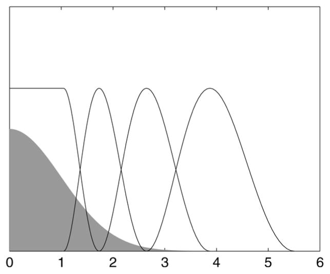
α, and β are chosen to map the centers of the second and last bump to $\sqrt{3}\sigma$ and $\sqrt{15}\sigma$, respectively. The first bump is altered to continue as a constant to the left of the peak (see Fig. 1), providing the denoiser with the capability to eliminate small amplitude coefficients. This family can generate smooth shrinkage functions, including linear estimators, as well as nonlinear “coring” estimators that approximate hard thresholding. In order to restrict the number of parameters that must be optimized, we limit the representation to four bumps, as illustrated in Fig. 1.

Fig. 1.

Linear basis of “bump” functions, b_k, used to form g_θ(y). Positions of these functions are adapted to the noise level: Abscissa units are in multiples of σ, the standard deviation of the corresponding Gaussian noise distribution, indicated by the gray region.

To test our methodology, we used decompositions based on a separable Haar basis [30], consisting of local averages and differences of adjacent local averages. These are the simplest (and oldest) of all wavelets, and are easily and efficiently implemented. We used the orthonormal basis, as well as an undecimated decomposition with periodic boundary extension. All images were decomposed into five dyadic scales, which means that the undecimated transform is overcomplete by a factor of 16.

B. Simulated Results

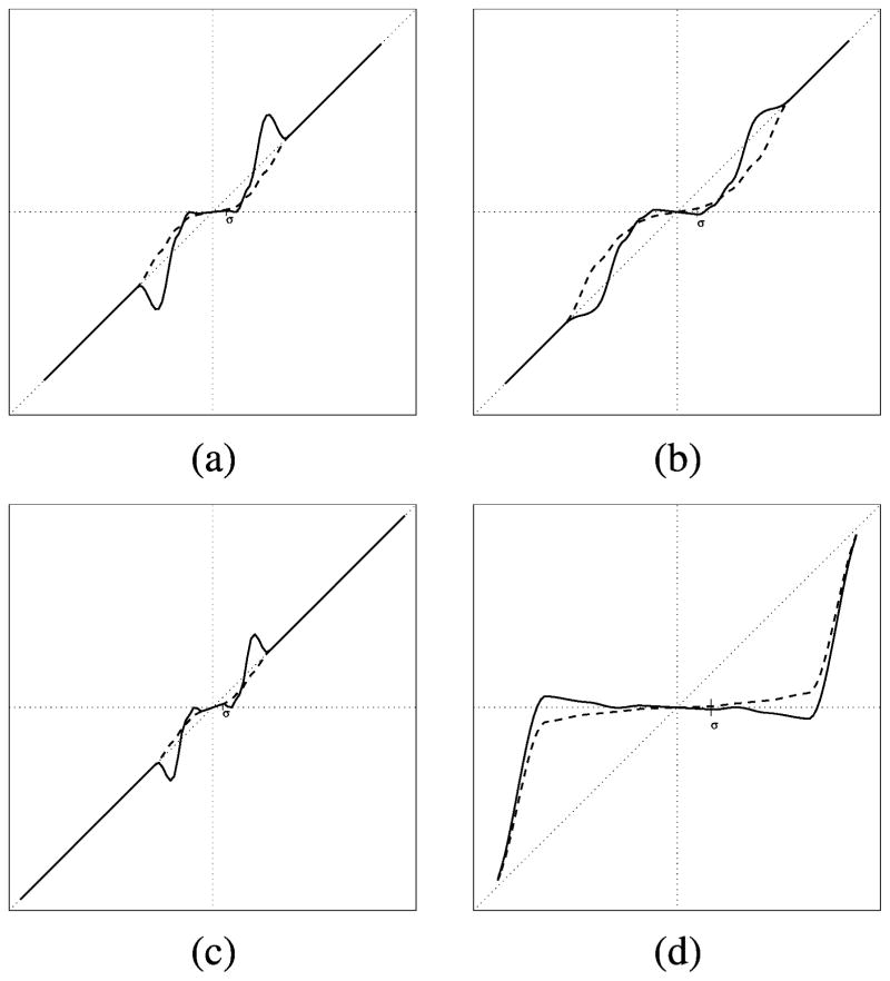
We computed optimal denoisers by optimizing SURE over the coefficients of the bumps basis, a method which we will refer to as SUREbumps. For the orthonormal case, we optimize (16), which is equivalent to (14). For the overcomplete (undecimated) case, we considered estimators optimized in the subband domain using (16) as well as estimators optimized in the image domain using (14). Fig. 2 shows a comparison of typical shrinkage functions that result from image-domain and subband-domain optimization. Roughly speaking, optimization in the image domain produces stronger suppression of small coefficients, along with preservation (or even boosting) of coefficients of moderate magnitude. That is, we may view the estimator as performing a type of sparsification, as suggested in [7] and [21]: lower-amplitude coefficients are suppressed, but medium-amplitude coefficients are boosted in order to compensate for the loss of signal energy. The boosting of mid-amplitude coefficients is also consistent with the findings of [13], in which linearly parameterized marginal shrinkage functions applied to an overcomplete block DCT representation were optimized for image-domain MSE by training on an ensemble of clean images.

Fig. 2.

Example shrinkage functions, x̂(y) = y + yΣg_θ(y), for various subbands of an undecimated Haar decomposition, as optimized for SURE in the subband domain (dashed line) and in the image domain (solid line). For midrange bands (a)–(c), the image-domain estimation functions show more shrinkage of low amplitude coefficients, with a compensatory amplification of midrange values. The high frequency band (d) shows more shrinkage. Note that all functions are equal to the identity for large values, beyond the location of the last bump.

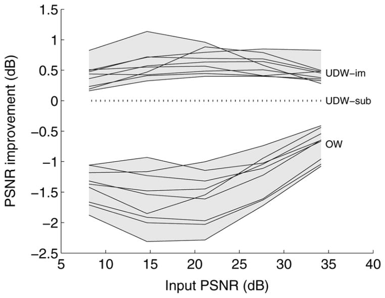
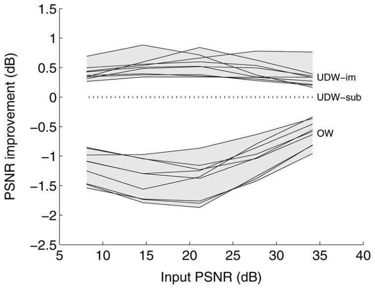
Fig. 3 shows a comparison of PSNR performance of three methods, across nine test images [12] and a wide range of noise levels. Consistent with the proof of Section II, and with empirical results of previous literature, we see that optimizing the denoiser in the subbands of the undecimated basis leads to significant improvement (typically 1.5 dB) over the orthonormal basis. Optimizing in the image domain leads to additional improvement (typically 0.5 dB).

Fig. 3.

Comparison of denoising results for scalar SUREbumps denoisers. Each group of lines (indicated by gray regions) shows results for one type of estimator. Each line within a group indicates improvement in PSNR, as a function of input PSNR, for one of nine denoised test images [12]. All results are shown relative to those of SUREbumps applied to undecimated Haar wavelets, optimized in the subband domain (dotted line). Bottom group: SUREbumps applied to orthogonal Haar wavelets. Top group: SUREbumps applied to undecimated Haar wavelets, optimized for image-domain MSE.

To give some indication of improvement compared to a well-known result in the literature, we also compared SUREbumps with SUREshrink [31], which is based on soft thresholding functions of the form:

$$g_{\theta }(y)=\{\begin{array}{ll}-y,\hfill & \mid y\mid \le \theta \hfill \\ -sgn(y)\theta ,\hfill & \mid y\mid >\theta .\hfill \end{array}$$

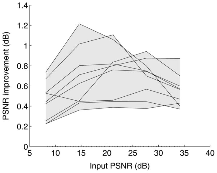
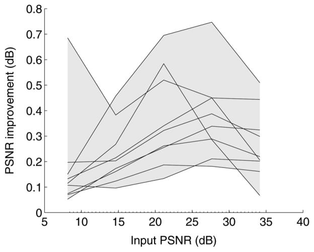
Although SUREshrink may be optimized for the image domain using (14), the resulting multidimensional objective function is nonconvex, and, thus, it is not feasible to guarantee global optimality of the solution. Thus, we optimize each threshold parameter θ_k independently by minimizing SURE over subband using (16), as was done in [19] and [31]. Fig. 4 shows a comparison across all test images and noise levels, demonstrating that SUREbumps optimized in the image domain offers a substantial improvement over SUREshrink in the transform domain (typically 0.6 dB).

Fig. 4.

Performance of SUREbumps optimized in the image domain, relative to SUREshrink (soft thresholding) optimized in the subband domain [19]. Both estimators are applied to coefficients of an undecimated Haar representation. Each line indicates improvement in PSNR (dB) for one of nine test images [12].

C. Image-Domain Optimization of Other Redundant Transforms

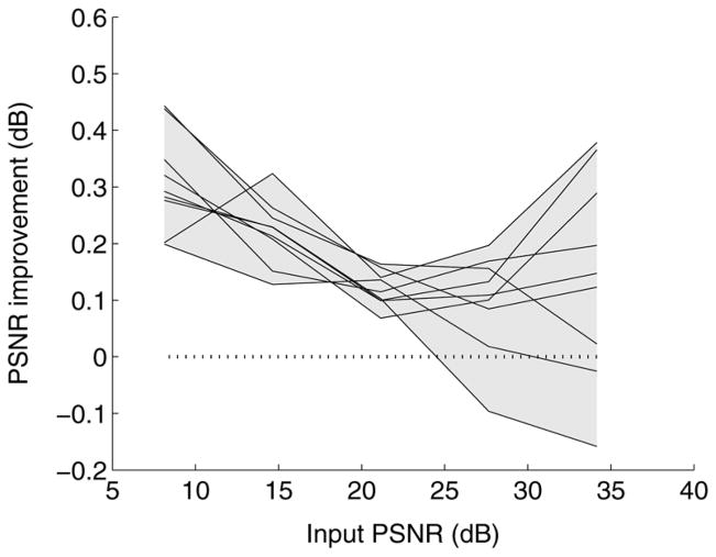
Thus far, we have shown examples with orthonormal and undecimated wavelet decompositions, which directly reveal the advantages of introducing redundancy, and of joint optimization in the image domain. However, our method for jointly optimizing the subband denoising functions is valid for any transform with a left inverse, and in particular for all tight frames. As such, we have also examined the behavior of SUREbumps when jointly optimizing estimators applied to a tight frame known as the “steerable pyramid” [23]. The representation is overcomplete by a factor of roughly 4K/3+1, where K is the number of orientation bands utilized. In our tests, we used K = 4, which produces a transform that is overcomplete by a factor of 6.33. Fig. 5 shows the improvement obtained by using SUREbumps in the image domain compared with SUREbumps in the subband domain. Significant improvement is still obtained, although not quite as much as in the undecimated wavelet case shown in Fig. 3, perhaps because the degree of overcompleteness is much less than for the undecimated wavelet representation. Also notice that at high noise levels (low PSNR), the pyramid-domain method sometimes outperforms the image-domain method. As mentioned earlier, this can arise from sampling errors in SURE, which have more of an effect when trying to jointly optimize the parameters for all the bands, instead of for each band separately.

Fig. 5.

Performance of SUREbumps estimators on a steerable pyramid decomposition, with five scales and four oriented subbands at each scale. Lines show performance of SUREbumps optimized in the image domain, relative to SUREbumps optimized in the subband domain.

V. Example: Local Context Estimators in Overcomplete Bases

As mentioned in Section II, substantial improvements can be achieved with estimators that operate on neighborhoods of coefficients. We previously defined context estimators in which each coefficient is denoised as a function of its surrounding neighbors, according to (4). Rewriting this in terms of g gives

$${\widehat{v}}_i({\mathbf{u}}_i)=u_i+g_k({\mathbf{u}}_i).$$ (19)

SURE can be extended to handle this situation, by taking into account the fact that coefficients are no longer denoised independently.

To simplify notation and computation, we assume that the neighborhood of each coefficient contains only coefficients from the same subband. Using our previous notation for the inner products of the transform basis functions, we can express the covariance structure of the noise within the subband as

$$C_{ij}={\sigma }^2{n}_{ij}.$$

Equation (7) implies that to denoise subband , we should pick g_k to minimize

$$\sum _{i\in {\mathcal{S}}_k}{g}_k{({\mathbf{U}}_i)}^2+2{\sigma }^2\sum _{i\in {\mathcal{S}}_k}{\mathbf{n}}_k·\nabla g_k({\mathbf{U}}_i)$$ (20)

where n_k is a vector that contains the inner product of the basis vector corresponding to the coefficient in the center of a neighborhood with every basis function in that neighborhood. Analogous to (16), the single-band expressions may be additively combined in a single objective function for optimizing the set {g_k} in the subband domain

$$\sum _k\sum _{i\in {\mathcal{S}}_k}{g}_k{({\mathbf{U}}_i)}^2+2{\sigma }^2\sum _k\sum _{i\in {\mathcal{S}}_k}{\mathbf{n}}_k·\nabla g_k({\mathbf{U}}_i)$$ (21)

On the other hand, if we wish to use SURE to denoise in the image domain, (13) implies we must choose {g_k} to minimize

$${\mid W^{T}g({\mathbf{U}}_i)\mid }^2+2{\sigma }^2\sum _k\sum _{i\in {\mathcal{S}}_k}{\mathbf{n}}_k·\nabla g_k({\mathbf{U}}_i).$$ (22)

As in the scalar case, the first term takes into account the interactions of the denoising operations when the coefficients are recombined in the image domain.

A. Implementation

Analogous to the 1-D case, we choose a linear family of estimators that operate by shrinking the noisy observation by a factor that depends on the amplitude of the observation relative to the noise strength

$$\widehat{\mathbf{V}}({\mathbf{U}}_i)={\mathbf{U}}_i+{\mathbf{U}}_i\sum _m{\theta }_m{b}_m\left(\sqrt{{\mathbf{U}}_i^T{C}_n^{-1}{\mathbf{U}}_i}\right)$$

where C_n is the noise covariance in the subband, and the bump functions b_k are defined as before by (18), except that the locations of the first and last bumps are scaled by the square root of the dimension. An example of the type of shrinkage field that results from this parameterization is shown for the 2-D case in Fig. 6. As described in (19), we then use this to denoise the central coefficient

Fig. 6.

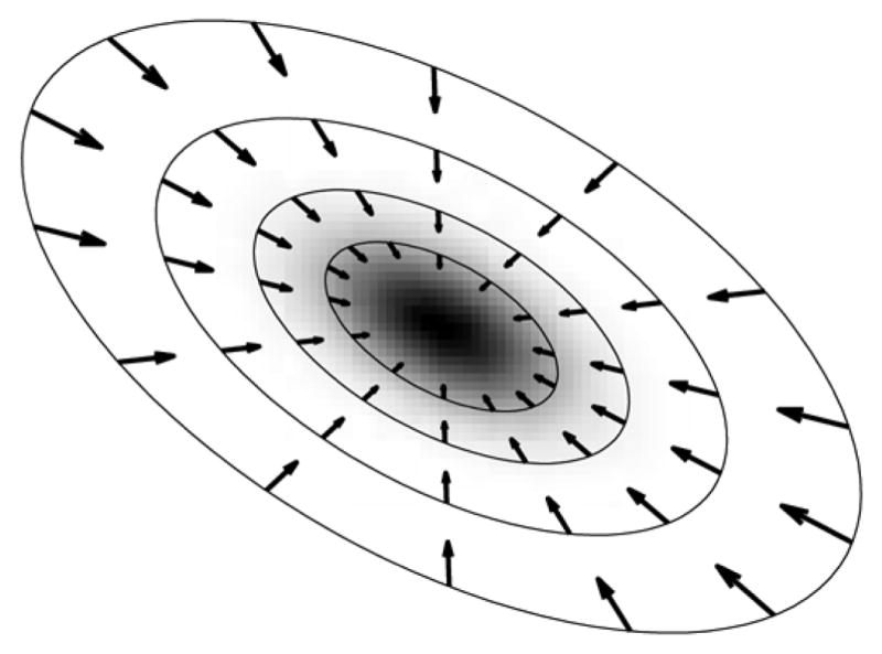
Illustration of joint shrinkage function, as a vector field in two dimensions, superimposed on a grayscale image representing the underlying Gaussian noise density. Each vector shows the change made to an observed (noisy) vector u. Elliptical contours indicate the maxima of the four bump functions, b_k. The set of vectors u that lie along any one of these contours are denoised by multiplying by a common scalar shrinkage factor. In practice, only the coefficient at the center of each neighborhood is multiplied by this factor.

$${\widehat{V}}_i({\mathbf{U}}_i)=U_i+U_i\sum _m{\theta }_m{b}_m\left(\sqrt{{\mathbf{U}}_i^T{C}_n^{-1}{\mathbf{U}}_i}\right).$$

To illustrate our theorem, we used spatial neighborhoods of size 3 × 3 coefficients, located on a subsampled lattice as described in Section II, and boundaries (including neighborhood calculations) are handled with periodic extension.

B. Simulation Results

Fig. 7 shows a performance comparison of the vector bumps denoiser optimized individually for subband-domain MSE [using (21)] and optimized jointly for image-domain MSE [using (22)]. As in the scalar case, and consistent with the proof of Section II, application of SUREbumps in the over-complete (undecimated) representation leads to a substantial improvement over application in the orthonormal representation (typically, >1dB), and optimization in the image domain offers an additional improvement over optimization in the subband domain (nearly 0.5 dB).

Fig. 7.

Comparison of denoising results for vector SUREbumps denoisers. See caption of Fig. 3.

C. Comparison of Vector and Scalar SUREbumps

Thus far, we used a neighborhood structure such that the basis vectors associated with the elements of a neighborhood are orthogonal. In this situation, examination of (22) shows that the MSE estimate is not much different from that of the marginal case, in that it does not make use of the derivative of the denoised coefficient with respect to its neighbors. Consistent with this, we find experimentally that a denoiser based on this neighborhood structure does not show much performance gain compared to a scalar denoiser. For these reasons, we have also implemented a vector denoiser based on neighborhood containing a 3 × 3 set of nearest neighbors on the undecimated lattice. Fig. 8 shows the improvement of this nearest-neighbor denoiser over the scalar denoiser, which is typically 0.1–0.5 dB.

Fig. 8.

Comparison of denoising results for vector SUREbumps (solid lines) relative to those for scalar SUREbumps. Both estimators are applied to an undecimated Haar decomposition and optimized in the image domain. This vector denoiser uses 3 × 3 neighborhoods of adjacent coefficients in the undecimated decomposition.

D. Comparison to BLS-GSM Context Denoiser

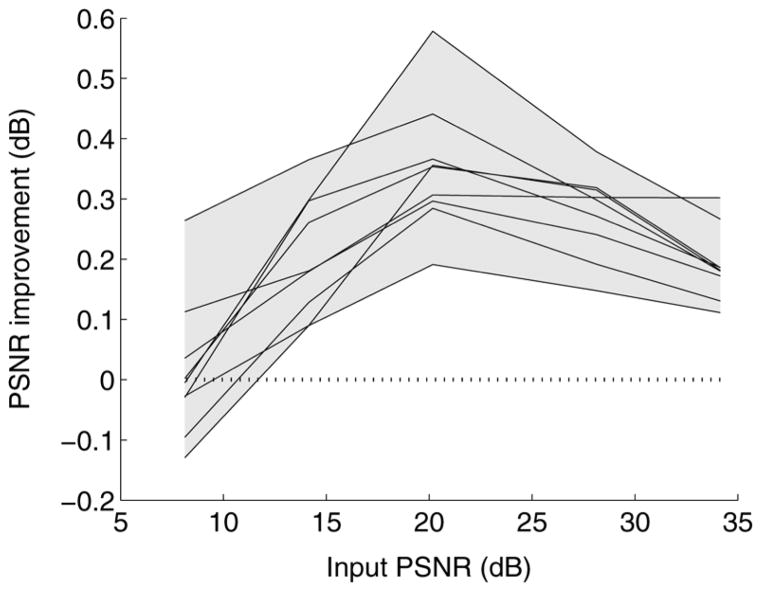
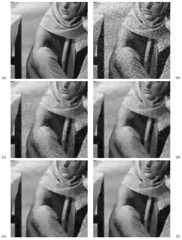
To give some indication of improvement relative to another result in the literature, we also applied the BLS-GSM estimator of [12] to the undecimated Haar decomposition using the same neighborhood structure. Note that the originally published BLS-GSM results use a steerable pyramid decomposition, reflected boundary handling, different neighborhood structure near the boundary, and include coarser-scale parents as part of the neighborhood. By enforcing the same decomposition and neighborhood structure, we are providing a direct comparison of the two statistical procedures: BLS-GSM, which is based on an explicit prior model, and SUREbumps, which is prior-free and based on an explicitly parameterized denoising function. Fig. 9 shows the improvement in PSNR of using the vector SUREbumps estimator optimized in the image domain, relative to using the BLS-GSM estimator. Despite the simplistic functional form of the estimator used in SUREbumps, performance is typically better than that of BLS-GSM. Table I provides PSNR values of the vector SUREbumps method, optimized in the image domain, for all test images at all noise levels. Although they do not quite achieve the performance level of current state-of-the-art methods (e.g., [28]), the results are roughly comparable to many recent results (e.g., [12], [32], [33], [34]), especially at low to moderate levels of noise. Fig. 10 shows example denoised images. Increases in redundancy and image domain optimization are both seen to improve visual quality.

Fig. 9.

Performance of vector SUREbumps optimized in the image domain, relative to BLS-GSM estimator [12] (dotted line). Both estimators are applied to coefficients of an undecimated Haar representation. Each line indicates improvement in PSNR (dB) for one of nine test images [12].

TABLE I.

Denoising Results for the Vector SUREbumps Method, for Nine Images at Five Different Noise Levels, Expressed as Peak-to-Peak Signal-to-Noise Ratio (PSNR). For All Results, SUREbumps Were Applied to a Five-Scale Undecimated Haar Decomposition, With 3 × 3 Neighborhood of Adjacent Coefficients, Optimized for Image-Domain MSE

σ/PSNR	Barbara	Boat	Flinstones	House	Lena	Goldhill	Tulips	Parkbench	Mtwill
5/34.15	37.13	37.21	35.93	38.84	38.38	37.08	38.58	35.98	36.53
10/28.13	33.01	33.69	31.92	35.63	35.24	33.43	34.73	31.33	32.77
25/20.17	27.88	29.42	27.53	31.75	31.19	29.45	30.14	26.10	28.82
50/14.15	24.41	26.34	24.02	28.15	28.18	26.85	26.75	23.05	26.13
100/8.13	22.20	23.64	20.29	24.50	25.28	24.48	23.51	20.62	23.60

Fig. 10.

Denoising results. (a) Original image (cropped); (b) noisy (15.00 dB); (c) scalar SUREbumps on orthogonal wavelet (22.96 dB); (d) scalar SUREbumps on undecimated wavelet, optimized in the subband domain (23.89 dB); (e) scalar SUREbumps on undecimated wavelet, optimized in the image domain (24.39 dB); (f) vector SUREbumps on undecimated wavelet, optimized in the image domain (24.86 dB). All methods are applied to a Haar decomposition.

VI. Discussion

In this paper, we have examined the problem of MSE-optimal denoising in overcomplete subband representations. We’ve provided a formal explanation for the empirically observed fact that subband denoising methods can be improved by making the representation more redundant, and we’ve shown that performance can be further improved by jointly optimizing the subband estimators to minimize image-domain MSE. In order to examine these effects empirically, we developed generalizations of Stein’s unbiased risk estimate to include correlated noise, vector denoisers, and image-domain MSE estimates for denoising functions applied to subbands of overcomplete representations. Using scalar and vector denoisers constructed from linear combinations of “bumps,” we have shown through simulations that optimization of image-domain MSE can lead to substantial performance gains over the suboptimal application of SURE in each subband. These results underscore the importance of distinguishing between the choice of subband decomposition (e.g., orthogonal versus redundant, separable versus oriented), the method of denoising (e.g., thresholding versus BLS-GSM versus linearly parameterized bumps), the means by which the denoiser parameters are selected (e.g., optimized over a training set versus maximum likelihood fitting of a prior density versus SURE) and the domain in which the parameters are optimized (subband versus image). Comparison of methods that differ in more than one of these factors leaves one unable to conclusively determine the underlying sources of advantage or disadvantage. While it is difficult to formally quantify the interaction of these factors, we believe such understanding would allow for further improvement in performance.

In order to simplify our presentation, we have focused on denoisers operating on rather simple decompositions (Haar wavelets with periodic boundary handling). These decompositions can easily be extended to form overcomplete tight frames by cycle-spinning or eliminating decimation. It is worth investigating the effects of overcompleteness in other bases, particularly oriented redundant tight frames (e.g., steerable pyramid [23], complex wavelets [25], curvelets [24]). In these cases, it might also prove worthwhile to explore other means of increasing redundancy, such as including rotated or dilated copies of the initial basis set into the transform. If the statistics of subbands are maintained when this redundancy is introduced, the proof of Section II will still guarantee improvement for transform domain denoising. Bases that use reflected boundary handling (as opposed to periodic handling) would also likely lead to improvements in performance [12]. Another issue worth investigating is the choice of neighborhoods on the performance of context denoisers. For example, the inclusion of coefficients from other subbands (e.g., coarser-scale “parents”) in the neighborhood has been found to produce substantial increases in performance [11], [12], [15], although a significant portion of these increases may be obtained through the use of larger spatial neighborhoods [35], [36].

Perhaps more importantly, we believe there is room for substantial improvement in the design of the denoising functions. The examples in this article used a fixed linear family of “bump” functions, whose shapes and positions were crudely hand-optimized to deal with several issues that can affect MSE. First, as in all statistical regression problems, the complexity of the model governs a well-known tradeoff between systematic errors (bias) and generalization errors (variance, or overfitting). Specifically, the family of denoising functions should be sufficiently rich to handle a wide variety of source images and noise levels, but it should also be simple enough that its parameters are well constrained by the observed image data. Errors in parameter estimation arise from errors in computing SURE, and these, in turn, depend on both the amount of data (e.g., the number of coefficients in a subband), and the strength of the signal relative to the noise. Second, the choice of denoiser need not rely entirely on the data from the particular image being denoised. Generally, denoising methods include some aspects that are tuned/adapted to the idiosyncrasies of each particular image, and other aspects that are chosen/optimized for performance over image ensembles. In fact, some methods rely entirely on the latter, optimizing over a large set of training images to select a single universal denoiser (e.g., [13], [33]). In our implementation, some prior information is implicitly included through the design of the bumps. Prior information could be more explicitly incorporated in the deterministic choice of a function family, and/or through a prior probability model on the parameter values. A principled solution should then trade off between adaptively optimizing for a particular image, whenever the data provide a sufficient constraint, and using the prior information to regularize the solution in cases for which the image data are insufficient.

More generally, the use of SURE for adapting a denoiser to the properties of an observed noisy sample is a particular solution of the “universal” restoration problem, which aims to recover a signal with unknown characteristics from observations corrupted by a process with known characteristics. This problem has been recently explored in several very different forms [27], [28], [29], [37], [38], [39], and it should prove interesting to explore the similarities and relative advantages of these methods.

Biographies

Eero P. Simoncelli (S’92–M’93-SM’04) received the B.S. degree (summa cum laude) in physics in 1984 from Harvard University, Cambridge, MA. He studied applied mathematics at Cambridge University, Cambridge, U.K., for a year and a half, and then received the M.S. and the Ph.D. degrees in electrical engineering from the Massachusetts Institute of Technology, Cambridge, MA, in 1988 and 1993, respectively.

He was an Assistant Professor of computer and information science, University of Pennsylvania, Philadelphia, from 1993 until 1996. He joined New York University in September of 1996, where he is currently a Professor of neural science and mathematics. In August 2000, he became an Investigator of the Howard Hughes Medical Institute, New York University, under their new program in Computational Biology. His research interests span a wide range of topics in the representation and analysis of visual images, in both machine and biological systems.

Martin Raphan (S’07–M’07) received the B.E. and M.E. degrees in electrical engineering from the Cooper Union for the Advancement of Science and Art, New York, in 2001 and 2003, respectively, and the M.A. and Ph.D. degrees in mathematics from the Courant Institute of Mathematical Sciences, New York University (NYU), in 2003 and 2007, respectively.

He is currently a Postdoctoral Fellow supported by the Howard Hughes Medical Institute, NYU.

Dr. Raphan received an IBM Student Paper Award at ICIP 2007. His doctoral dissertation, on prior-free methods of Bayesian estimation with applications to image processing and neuroscience, received the Kurt O. Friedrichs Prize for an outstanding dissertation in mathematics.

References

- 1.Rossi JP. Digital techniques for reducing television noise. JSMPTE. 1978;87:134–140. [Google Scholar]
- 2.Donoho D. Denoising by soft-thresholding. IEEE Trans Inf Theory. 1995 May;41(3):613–627. [Google Scholar]
- 3.Simoncelli EP, Adelson EH. Noise removal via Bayesian wavelet coring. Proc. 3rd IEEE Int. Conf. Image Processing; Lausanne, Switzerland. Sep. 16–19, 1996; pp. 379–382. [Google Scholar]
- 4.Chipman HA, Kolaczyk ED, McCulloch RM. Adaptive Bayesian wavelet shrinkage. J Amer Statist Assoc. 1997;92(440):1413–1421. [Google Scholar]
- 5.Abramovich F, Sapatinas T, Silverman BW. Wavelet thresholding via a Bayesian approach. J Roy Statist Soc B. 1998;60:725–749. [Google Scholar]
- 6.Vidakovic B. Nonlinear wavelet shrinkage with Bayes rules and Bayes factors. J Amer Statist Assoc. 1998;93:173–179. [Google Scholar]
- 7.Hyvarinen Sparse code shrinkage: Denoising of nongaussian data by maximum likelihood estimation. Neural Comput. 1999;11(7):1739–1768. doi: 10.1162/089976699300016214. [DOI] [PubMed] [Google Scholar]
- 8.Figueiredo M, Nowak R. Wavelet-based image estimation: An empirical Bayes approach using Jeffrey’s noninformative prior. IEEE Trans Image Process. 2001 Sep;10(9):1322–1331. doi: 10.1109/83.941856. [DOI] [PubMed] [Google Scholar]
- 9.Mihçak MK, Kozintsev I, Ramchandran K, Moulin P. Low-complexity image denoising based on statistical modeling of wavelet coefficients. Signal Process Lett. 1999 Dec;6(12):300–303. [Google Scholar]
- 10.Chang SG, Yu B, Vetterli M. Spatially adaptive wavelet thresholding with context modeling for image denoising. IEEE Trans Image Process. 2000 Sep;9(9):1522–1531. doi: 10.1109/83.862630. [DOI] [PubMed] [Google Scholar]
- 11.Şendur L, Selesnick IW. Bivariate shrinkage functions for wavelet-based denoising exploiting interscale dependency. IEEE Trans Signal Process. 2002 Nov;50(11):2744–2756. [Google Scholar]
- 12.Portilla J, Strela V, Wainwright MJ, Simoncelli EP. Image denoising using a scale mixture of Gaussians in the wavelet domain. IEEE Trans Image Process. 2003 Nov;12(11):1338–1351. doi: 10.1109/TIP.2003.818640. [DOI] [PubMed] [Google Scholar]
- 13.Hel-Or Y, Shaked D. A discriminative approach for wavelet denoising. IEEE Trans Image Process. 2008 Apr;17(4):443–457. doi: 10.1109/TIP.2008.917204. [DOI] [PubMed] [Google Scholar]
- 14.Stein CM. Estimation of the mean of a multivariate normal distribution. Ann Statist. 1981 Nov;9(6):1135–1151. [Google Scholar]
- 15.Luisier F, Blu T, Unser M. A new SURE approach to image denoising: Interscale orthonormal wavelet thresholding. IEEE Trans Image Process. 2007 Mar;16(3):593–606. doi: 10.1109/tip.2007.891064. [DOI] [PubMed] [Google Scholar]
- 16.Pesquet JC, Leporini D. A new wavelet estimator for image denoising. Proc. 6th Int. Conf. Image Processing and its Applications; Dublin, Ireland. Jul. 1997; pp. 249–253. [Google Scholar]
- 17.Benazza-Benyahia A, Pesquet JC. Building robust wavelet estimators for multicomponent images using Stein’s principle. IEEE Trans Image Process. 2005 Nov;14(11):1814–1830. doi: 10.1109/tip.2005.857247. [DOI] [PubMed] [Google Scholar]
- 18.Blu T, Luisier F. The SURE-LET approach to image denoising. IEEE Trans Image Process. 2007 Nov;16(11):2778–2786. doi: 10.1109/tip.2007.906002. [DOI] [PubMed] [Google Scholar]
- 19.Coifman RR, Donoho DL. Translation-invariant denoising. In: Antoniadis A, Oppenheim G, editors. Wavelets and Statistics. San Diego, CA: Springer-Verlag; 1995. [Google Scholar]
- 20.Simoncelli EP. Bayesian denoising of visual images in the wavelet domain. In: Müller P, Vidakovic B, editors. Bayesian Inference in Wavelet Based Models. Vol. 141. New York: Springer-Verlag; 1999. pp. 291–308. ch. 18. [Google Scholar]
- 21.Elad M. Why simple shrinkage is still relevant for redundant representations? IEEE Trans Inf Theory. 2006 Dec;52(12):5559–5569. [Google Scholar]
- 22.Raphan M, Simoncelli EP. Optimal denoising in redundant bases. presented at the 14th IEEE Int. Conf. Image Processing; San Antonio, TX. Sep. 2007; [DOI] [PMC free article] [PubMed] [Google Scholar]
- 23.Simoncelli EP, Freeman WT, Adelson EH, Heeger DJ. Shiftable multi-scale transforms. IEEE Trans Inf Theory. 1992 Mar;38(2):587–607. [Google Scholar]
- 24.Candès EJ, Donoho DL. Curvelets—A surprisingly effective nonadaptive representation for objects with edges. In: Rabut C, Cohen A, Schumaker LL, editors. Curves and Surfaces. Nashville, TN: Vanderbilt Univ. Press; 2000. pp. 105–V120. [Google Scholar]
- 25.Kingsbury N. Complex wavelets for shift invariant analysis and filtering of signals. Appl Comput Harmon Anal. 2001 May;10(3):234–253. [Google Scholar]
- 26.Fan G, Xia XG. Image denoising using a local contextual hidden Markov model in the wavelet domain. IEEE Signal Process Lett. 2001 May;8(5):125–128. [Google Scholar]
- 27.Buades A, Coll B, Morel JM. A review of image denoising algorithms, with a new one. Multiscale Model Simul. 2005 Jul;4(2):490–530. [Google Scholar]
- 28.Dabov K, Foi A, Katkovnik V, Egiazarian K. Image denoising by sparse 3D transform-domain collaborative filtering. IEEE Trans Image Process. 2007 Aug;16(8):2080–2095. doi: 10.1109/tip.2007.901238. [DOI] [PubMed] [Google Scholar]
- 29.Raphan M, Simöncelli EP. Learning to be Bayesian without supervision. In: Scholkopf B, Platt J, Hofmann T, editors. Adv Neural Information Processing Systems. Vol. 19. Vol. 19 Cambridge, MA: MIT Press; May, 2007. [Google Scholar]
- 30.Haar A. Zur theorie der orthogonalen funktionensysteme. Math Annal. 1910;69:331–371. [Google Scholar]
- 31.Donoho D, Johnstone I. Adapting to unknown smoothness via wavelet shrinkage. J Amer Statist Assoc. 1995 Dec;90(432) [Google Scholar]
- 32.Pižurica A, Philips W, Lemahieu I, Acheroy M. A joint inter- and intrascale statistical model for Bayesian wavelet based image denoising. IEEE Trans Image Process. 2002 May;11(5):545–557. doi: 10.1109/TIP.2002.1006401. [DOI] [PubMed] [Google Scholar]
- 33.Roth S, Black M. Fields of experts: A framework for learning image priors. Proc. IEEE Conf. Computer Vision and Pattern Recognition; Jun. 2005; pp. 860–867. [Google Scholar]
- 34.Kervrann C, Boulanger J. Optimal spatial adaptation for patch-based image denoising. IEEE Trans Image Process. 2006 Oct;15(10):2866–2878. doi: 10.1109/tip.2006.877529. [DOI] [PubMed] [Google Scholar]
- 35.Liu J, Moulin P. Information-theoretic analysis of interscale and intrascale dependencies between image wavelet coefficients. IEEE Trans Image Process. 2001 Nov;10(10):1647–1658. doi: 10.1109/83.967393. [DOI] [PubMed] [Google Scholar]
- 36.Buccigrossi RW, Simoncelli EP. Image compression via joint statistical characterization in the wavelet domain. IEEE Trans Image Process. 1999 Dec;8(12):1688–1701. doi: 10.1109/83.806616. [DOI] [PubMed] [Google Scholar]
- 37.Weissman T, Ordentlich E, Seroussi G, Verdú S, Weinberger M. Universal discrete denoising: Known channel. IEEE Trans Inf Theory. 2005 Jan;51(1):5–28. [Google Scholar]
- 38.Awate SP, Whitaker RT. Unsupervised, information-theoretic, adaptive image filtering for image restoration. IEEE Pattern Anal Mach Intell. 2006 Mar;28(3):364–376. doi: 10.1109/TPAMI.2006.64. [DOI] [PubMed] [Google Scholar]
- 39.Elad M, Aharon M. Image denoising via sparse and redundant representations over learned dictionaries. IEEE Trans Image Process. 2006 Dec;15(12):3736–3745. doi: 10.1109/tip.2006.881969. [DOI] [PubMed] [Google Scholar]