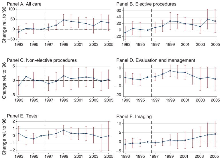
Figure 5. Supply Response by Service Category.

Notes: These graphs show coefficients and associated bootstrap standard errors from ordinary least squares regressions in which the quantities of health care supplied in different categories (as measured in Relative Value Units) are the dependent variables. These quantities are regressed on reimbursement rate shocks resulting from the consolidation of Medicare's fee schedule areas in 1997, as interacted with indicator variables for each year. These regressions are run at the payment area level after partialing out the following controls, as described in Section IB, and coefficients correspond to θ_p parameters in equation (3): county fixed effects, state-by-year effects, a set of year dummy variables interacted with each county's 1990 urban population share and an indicator for metropolitan status, the fraction of beneficiaries aged 65–59, 70–74, 75–79, and 80–84, black, Hispanic, female, eligible for Medicare due to end-stage renal disease or due to disability, with 2 or more, 3 or more, 4 or more, and 6 or more comorbidities as defined by Elixhauser et al. (1998). Standard errors are calculated with the bootstrap from online Appendix B.1.

Sources: Price change: Federal Register, various issues; Medicare claims data: Medicare Research Identifiable Files, 5 percent sample, described in Section IC; demographics: Ruggles et al. (2010).