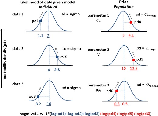
Fig. 4.

Maximum likelihood estimation for Bayes forecasting. A population pharmacokinetic model with three population parameters (CL, V, and KA) is available for a drug. Three concentration data points are available in a patient given the drug. In Bayes forecasting, a curve-fitting algorithm tries various individual values of CL, V, and KA for the patient to find the minimum value of the Bayes objective function. There are two components of the objective function—one that expresses the difference between the model predicted concentration and the observed concentration data (left column) and one that expresses the difference between the population values of CL, V, and KA and the current model estimate for the individual parameters (right column). The plots show the probability density distribution for each case (assuming a normal distribution). For the left column, each distribution is centered on the model predicted concentration and has variability described by sigma, the residual variability of the population model. The probability density for each observed data point is calculated—the better the fit of the data, the closer each data point is the center of the distribution. For the right column, each distribution is centered on the population parameter value and has variability described by omega, the previously observed variability of the parameter within the population. The probability density for current individual parameter values is calculated—the closer each individual parameter value is to the center of their distribution, the more the patient is considered to be consistent with the previously observed population. The objective function is derived from the product of all the probability density values shown. For computational convenience, the objective function is the negative log likelihood as shown