

Abstract
Motivation: The discovery of CRISPR-Cas systems almost 20 years ago rapidly changed our perception of the bacterial and archaeal immune systems. CRISPR loci consist of several repetitive DNA sequences called repeats, inter-spaced by stretches of variable length sequences called spacers. This CRISPR array is transcribed and processed into multiple mature RNA species (crRNAs). A single crRNA is integrated into an interference complex, together with CRISPR-associated (Cas) proteins, to bind and degrade invading nucleic acids. Although existing bioinformatics tools can recognize CRISPR loci by their characteristic repeat-spacer architecture, they generally output CRISPR arrays of ambiguous orientation and thus do not determine the strand from which crRNAs are processed. Knowledge of the correct orientation is crucial for many tasks, including the classification of CRISPR conservation, the detection of leader regions, the identification of target sites (protospacers) on invading genetic elements and the characterization of protospacer-adjacent motifs.
Results: We present a fast and accurate tool to determine the crRNA-encoding strand at CRISPR loci by predicting the correct orientation of repeats based on an advanced machine learning approach. Both the repeat sequence and mutation information were encoded and processed by an efficient graph kernel to learn higher-order correlations. The model was trained and tested on curated data comprising >4500 CRISPRs and yielded a remarkable performance of 0.95 AUC ROC (area under the curve of the receiver operator characteristic). In addition, we show that accurate orientation information greatly improved detection of conserved repeat sequence families and structure motifs. We integrated CRISPRstrand predictions into our CRISPRmap web server of CRISPR conservation and updated the latter to version 2.0.
Availability: CRISPRmap and CRISPRstrand are available at http://rna.informatik.uni-freiburg.de/CRISPRmap.
Contact: backofen@informatik.uni-freiburg.de
Supplementary information: Supplementary data are available at Bioinformatics online.
1 INTRODUCTION
CRISPR-Cas immune systems of bacteria and archaea provide adaptive defence against a variety of invading genetic elements. They have been classified into three major classes: Types I, II and III, where Type II systems are confined to bacteria (Makarova et al., 2011a; Vestergaard et al., 2014). The adaptive immune response of all types is divided into three major phases: (i) adaptation, the uptake of DNA fragments from genetic elements and their insertion between consecutive repeats of a CRISPR array, generally adjacent to a leader sequence; (ii) processing of the CRISPR array transcripts within the repeats to generate small crRNAs that derive from part or all of each spacer region and (iii) interference involving targeting and cleavage of an invading genetic element, or its transcripts, by Cas protein–crRNA complexes (Barrangou and van der Oost, 2013, and Fig. 1). Whereas the adaptation phase is relatively conserved in the different CRISPR-Cas systems, significant differences occur in the processing and interference mechanisms. Thus, where Type I and III systems employ a Cas6 processing endonuclease to cleave within the repeats, the bacterial Type II system uses the host-encoded RNase III, together with a CRISPR-associated, trans-encoded tracrRNA (Deltcheva et al., 2011). Furthermore, the various interference complexes exhibit considerable diversity (Barrangou and van der Oost, 2013; Makarova et al., 2011a; Vestergaard et al., 2014).
Fig. 1.

The three major phases of CRISPR-Cas immune systems. First, in the adaptation phase, Cas proteins excise the protospacer sequence from foreign DNA and insert it into the repeat, adjacent to the leader at the CRISPR locus. Second, CRISPR arrays are transcribed and then processed into multiple crRNAs, each carrying a single spacer sequence and part of the adjoining repeat sequence. Third, at the interference phase, the crRNAs are assembled into different classes of protein targeting complexes (Cascades) that anneal to, and cleave, spacer matching sequences on either invading element or their transcripts
We developed an efficient tool for determining the strand from which mature crRNAs are derived by focussing on the repeats at CRISPR loci. The repeats are unique within the CRISPR-Cas system because they are the only element to play a vital role in all phases of immunity (Barrangou and van der Oost, 2013). Thus, despite their relatively short lengths, each repeat carries essential structural parameters or sequence motifs that are recognized by enzymes or structural proteins involved in adaptation, crRNA biogenesis and interference. Paradoxically, however, the repeats are very heterogeneous, occurring in a range of lengths, 19–48 nt, and display considerable sequence diversity. An early comparative study of CRISPR diversity yielded 12 main clusters with specific sequence characteristics; only a subset folded into characteristic hairpin structure motifs (Kunin et al., 2007). More recently, a major reevaluation of CRISPR conservation was executed by Lange et al. (2013), on a much larger data set of 3527 CRISPRs, where 40 conserved repeat sequence families were identified together with a total of 33 potential structural motifs. The repeat clusters were further classified into six superclasses, some of which showed strong biases to specific CRISPR subtypes and to certain bacterial or archaeal phyla (Lange et al., 2013).
CRISPR loci are generally identified by their characteristic repeat-spacer architecture. For example CRT (Bland et al., 2007) and CRISPRFinder (Grissa et al., 2007) provide sensitive predictions of CRISPR arrays, but do not provide unambiguous orientation information. In the literature, orientation is derived mainly by characteristic sequence motifs in the repeat, the detection of a conserved leader region in closely related CRISPR loci or by transcriptome experiments where the dominantly transcribed strand is determined. However, to date very few systems have been studied experimentally, and many large-scale studies require accurate orientation information for all available CRISPR arrays. Recently, Biswas et al. (2014) has presented the first tool to predict the orientation of CRISPR arrays. Their model is essentially a linear predictor based on a number of features which comprise the presence of the ATTGAAAN motif in repeats, a higher A or T content in the flanking regions of CRISPR arrays, nucleotide composition within the CRISPR array, the presence of mutations in specific parts of the array and the tendency to fold into a secondary structure. Each feature is considered as an independent predictor and is given a weight proportional to its estimated precision. The final prediction is computed as the weighted combination of each predictor.
Knowledge of the correct repeat orientation is crucial for accurate characterization of CRISPR conservation and for subsequently studying mechanisms of adaptation, CRISPR RNA processing and interference. In particular, it can help to (i) detect leader regions, currently poorly described in the literature; (ii) identify signals of transcription initiation and termination; (iii) determine the orientation of protospacers on invading genetic elements; and finally, (iv) characterize cognate protospacer-adjacent motifs (PAMs). Thus, we consider that the repeat orientation tool presented here will be of critical importance for future CRISPR-based experimental studies.
2 MATERIALS AND METHODS
We present a linear discriminative model based on graph kernels to accurately predict the orientation of the CRISPR sequence. The method first generates a sequence alignment of all repeat instances in the CRISPR array and outputs the consensus repeat sequence in its predicted orientation and whether it lies on the forward or reverse strand. There are two core ideas underlying our approach. The first one is to use a combinatorial technique to extract a very large number of features. The second idea is to encode our knowledge about the problem as a directed graph with discrete labels. The first idea allows a predictive system to be very accurate and to express complex discriminative decisions; the second idea allows a natural and flexible encoding of background knowledge.
2.1 Novel comprehensive identification of CRISPR loci
We extracted a comprehensive dataset of CRISPR loci from published archaeal and bacterial genomes. All genome sequences were downloaded from the NCBI website (http://www.ncbi.nlm.nih.gov/). We predicted CRISPR loci using CRISPRFinder (Grissa et al., 2007) and CRT (Bland et al., 2007). For both tools, we used (i) default parameter values for predicted CRISPR loci and (ii) parameters that corresponded to at least two repeats within a CRISPR locus; repeat and spacer lengths were set to a range between 18 and 78 bp. We then (iii) generated a consensus repeat for each CRISPR locus exploiting the fact that repeats within a CRISPR locus are almost completely identical with some loci that carry few mutations, preferably at the start and end (see Supplementary Figure S3, Supplementary material). Because CRT does not output consensus repeats, we used the MAFFT program (Katoh et al., 2002), version 6.4., to compute the multiple alignments and the Cons program from EMBOSS package (Rice et al., 2000) to obtain the consensus repeat from the multiple sequence alignments. Finally, (iv) the results from both CRISPRFinder and CRT tools were merged and redundant CRISPR loci were removed. In this way, we obtained a CRISPR databases with >4700 consensus repeats, which we refer to as REPEATS (see Table 1 for details).
Table 1.
Summary of our REPEATS dataset derived from all available CRISPR loci
| Data statistics | Archaea | Bacteria | ||
|---|---|---|---|---|
| Genomes (total) | 309 | 4590 | (4899) | |
| Genomes with CRISPRs (%) | 217 | (70) | 1409 | (30) |
| CRISPRs on forward strand | 516 | 1810 | (2326) | |
| CRISPRs on reverse strand | 530 | 1859 | (2389) | |
| Repeats per array (median) | 2–198 | (20) | 2–1371 | (16) |
| Repeat lengths (median) | 20–44 | (29) | 19–48 | (30) |
| Spacer lengths (median) | 20–54 | (38) | 19–72 | (35) |
2.2 Datasets from literature
2.2.1 Set of repeats from Lange et al. (2013)
We selected structural motifs that fit to known cleavage sites (Lange et al., 2013). Table 2 gives a summary of published CRISPR-Cas systems with experimental evidence for the processing mechanism which we refer to as REPEATSLange. This dataset contains 324 bacterial and 118 archaeal repeat sequences (442 in total).
Table 2.
Summary of REPEATSLange dataset: published CRISPR-Cas systems with experimental evidence of the processing mechanism
| Organism | Motif | Cas subtype | Summary |
|---|---|---|---|
| Escherichia coli K12 | M2 | I-E | Structure predicted, but stable; 8-nt-5′-tag; cleavage by Cas6e, biochemical experiments (Brouns et al., 2008) |
| Thermus thermophilus HB8 | M2 | I-E | Structured; 8-nt-5′-tag; cleavage by Cas6e; crystal structure of repeat hairpin in Cas6e (Cse3) (Gesner et al., 2011; Juranek et al., 2012; Sashital et al., 2011) |
| Bacillus halodurans C-125 | M3 | I-C | Cleavage by Cas5d; 11-nt-5′-tag mutational analysis of hairpin structure (Nam et al., 2012) |
| Pseudomonas aeruginosa UCBPP-PA14 | M4 | I-F | Cleavage by Cas6f (Csy4); 8-nt-5′-tag; crystal structure and mutational analyses of repeat hairpin in Cas6f (Haurwitz et al., 2010, 2012; Sternberg et al., 2012) |
| Synechocystis sp. PCC6803 | M5 | I-DIII-variant | Cleavage by Cas6; 8-nt-5′-tag; biochemical experiments, extended structure prediction of hairpin motif (Scholz et al., 2013) |
| Thermus thermophilus HB27 | M9 | I-C | Cleavage by Cas5d; 11-nt-5′-tag biochemical experiments (Garside et al., 2012) |
| Methanosarcina marzei Gö1 | M13 | I-B III-B | Cleavage by Cas6b; 8-nt-5′-tag; structure probing experiment of hairpin (Nickel et al., 2013) |
| Synechocystis sp. PCC6803 | M14 | III-variant | Biochemical analysis of Cmr2 implicate its involvement in either cleavage, crRNA stabilization, or array expression regulation; 13-nt-5′-tag (Scholz et al., 2013) |
| Staphylococcus epidermidis RP62A | M28 | III-A | Cleavage by Cas6; 8-nt-5′-tag; hairpin structure as in M28 verified by mutational analysis and sequence specificity around cleavage site (Hatoum-Aslan et al., 2011) |
| Methanococcus maripaludis C5 | M29 | I-B | Cleavage by Cas6b; 8-nt-5′-tag; biochemical experiments (Richter et al., 2012) |
Note: In particular, these are systems for which (i) the Cas endoribonuclease has been characterized and/or (ii) the repeat structure has been verified. Published results are consistent with the data of Lange et al. (2013).
2.2.2 Set of repeats from Kunin et al. (2007)
We denote the dataset originally published in Kunin et al. (2007) as REPEATSKunin. The dataset contains 327 bacterial and 92 archaeal repeat sequences (419 in total). The orientations were assigned by the authors using previously published sequence features.
2.2.3 Set of archaeal repeats from Shah and Garrett (2011)
We denote the dataset based on the results available in (Shah and Garrett, 2011) as REPEATSShah. This dataset contains 478 archaeal repeat sequences with manually verified strand orientation.
2.3 Encoding CRISPR repeats as graphs
The features used to discriminate between the different orientation are based on available biological knowledge of CRISPR evolution and processing. During CRISPR RNA processing by Cas6-like endoribonucleases, cleavage occurs either at the -end base of the hairpin motif, or within the double-stranded region of the hairpin stem, usually below a base pair (Barrangou and van der Oost, 2013; Richter et al., 2012; Scholz et al., 2013). The product of this cleavage is an 8-nt-long AUUGAAA(N) repeat tag at the 5′-end of the mature crRNA (5′-tag), which corresponds to the last eight nucleotides from the 3′-end of the repeat sequence. Kunin et al. (2007) and Lange et al. (2013) showed that in some cases the four nucleotides AAA(N) motif can be used to identify the orientation. These observations lead to the hypothesis that the terminal region of the sequence, comprising four or eight nucleotides, plays a key role. We observed also that the mutation rate in various parts of the CRISPR locus is non-uniform, in particular the middle part of the CRISPR locus is more conserved. This finding motivated the idea of using the presence of mutations as an additional signal to detect the predominantly transcribed strand.
We made use of this background knowledge to partition the consensus repeat into specific informative parts: we distinguish terminal regions of identical size k at both ends (as the correct orientation is unknown) and a central variable length area. The terminal sequences are further partitioned into P equally sized parts, where we expect to find key motifs. We call each part block. One of the main signals that we used to define the number and size of the blocks is the mutation rate, defined as the fraction of mutations per nucleotide in each block. In Supplementary Figure S3, we report the mutation rate for the CRISPR locus partitioning with k = 8 and P = 2 on a dataset of 897 CRISPR arrays (Kunin et al., 2007; Shah and Garrett, 2011): each repeat is split into five adjacent regions, with terminal blocks spanning exactly 4 nucleotides and a central block spanning 12 nucleotides on average. In these settings, we observed a highly significant 4-fold and a 16-fold increase in the mutation rate in the initial 8 nucleotides and in the terminal block, respectively, as compared to the middle block. In Section 3.1, we have further validated the optimality of this partitioning with in silico simulations.
We encoded all our intuitions and knowledge on the relevant signals that a predictive model should be aware of in a graph data structure. The reason for this choice is 2-fold. First, we want an easy and natural way to inject different types of information in the problem solution, and, second, we want to exploit efficient techniques developed in the Machine Learning literature to automatically construct a large number of derived features to improve the accuracy of predictive models.
The graph formalism allows us, in a very natural and flexible way, to add knowledge by inserting informative entities as vertices and connecting them to the relevant parts of the current encoding via the edge notion. In our case, the information provided by the consensus sequence is modelled directly as a path graph with vertices labelled with the consensus nucleotide code (see Fig. 2). We then model the global localization information as additional vertices with a label that indicates the block identity. This reveals whether a nucleotide is located at the very beginning or just near the beginning of the sequence (and symmetrically for the opposite end). Furthermore, we consider a more fine grained localization information, identifying the specific position of a nucleotide within a block. The reason to encode an increasingly refined localization information is to allow the algorithm to choose the optimal level of detail needed in various parts of the sequence. Finally, the main piece of information is whether there is evidence of a mutation at a specific location; we model this with an additional vertex labelled with a binary code to indicate the presence of a mutation in at least one of the repeated sequences.
Fig. 2.
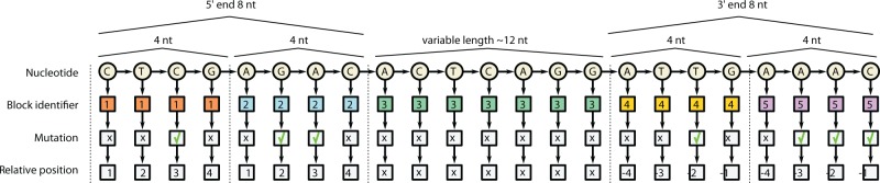
Graph encoding the consensus repeat sequence. The consensus nucleotide information is represented as a path graph, and additional information is modelled as a chain of additional vertices. The terminal parts of the repeat are marked with block identifiers
The final modelling decision regards the topology of the graph, i.e. how the additional vertices, which encode the different types of information, should be connected together. We identify an order which reflects the importance of the different types of information, starting from the nucleotide type, the block ID, the mutation evidence and finally the relative position within a block. Note that the combinatorial feature generation phase is affected by the sequential order of these attributes, as the information that is ranked higher will participate in the generation of more features and will therefore be regarded as more prominent.
2.4 Predictive model and feature extraction
After having encoded domain expert knowledge as a graph, we need to process this type of structured data to induce a predictive model. We do this using the technique developed by Costa and Grave (2010), based on the notion of graph kernels. The core idea (see Supplementary Information for a formal description) is to decompose each graph in a (multi) set of fragments and use these as features, in a similar fashion to what is done in the chemoinformatics domain with the fingerprint technique. The resulting sparse vectors can then be processed by efficient machine learning techniques, such as the stochastic gradient descent SVM (Bottou, 2010), to yield fast and highly predictive models. The type of graph decomposition that we use is called Neighbourhood Subgraph Pairwise Distance Kernel (NSPDK), and it involves the extraction of all possible pairs of small neighbourhood subgraphs that are not too distant (see Fig. 3). Intuitively one can think about this type of decomposition as an upgrade of the concept of k-mers with gaps from the domain of strings to that of graphs. Both the extraction of the features and the training of the predictive model have linear complexity and offer therefore excellent scaling capability. More precisely, extracting all neighbourhood subgraphs is achieved with a breadth-first visit for a limited depth starting from each node, and as the graphs are sparse, it takes where n is the number of nucleotides and m the number of repeat alignments.
Fig. 3.

The NSPDK approach extracts a large number of features taking only specific fragments into account. The procedure is parametrized by the radius R and the distance D. Each vertex is considered in turn as a root. A neighbourhood graph of radius R is extracted around each root. All possible pairs of neighbourhood graphs of the same size R are considered, provided that their respective roots are exactly at distance D. To understand the importance of the sequential order of the attributes consider the left part of the figure: here we depict a feature with radius 1 and distance 0, which will encode three pieces of information: (i) the specific dinucleotide combination, (ii) the block ID and (iii) whether a mutation is likely to occur on the first nucleotide of the dinucleotide. As we increase the maximal distance between the roots in the pair, the encoded information is further specialized. In the middle part of the figure, we show a feature that additionally includes the presence of a mutation at distance 5. When the radius is increased to 2, the specific position within the block is also considered
Finally, given that one of the two strands can be the one that exhibits a characteristic pattern, we train a predictive model on both variants of each repeat sequence: one obtained from the forward strand and the other from the complementary reverse strand. The binary task is therefore to assign a positive score to the sequences that are transcribed and a negative one to the complementary strand. In the predictive phase, we enforce consistency by considering the prediction on both variants of the sequence: a strong confidence of the prediction of the forward strand should also correspond to an equally confident prediction that the reverse complementary sequence is not transcribed. To do so, we simply perform the individual predictions and then average the prediction of the forward strand with the opposite prediction for the reverse strand. If the resulting score is positive, then the forward strand is predicted to be transcribed, whereas the reverse strand is selected if the score is negative.
3 RESULTS AND DISCUSSION
3.1 Parameter selection
We have previously described how relevant biological knowledge was used to determine various modelling choices. The proposed model admits, however, different configurations both in the encoding part as well as in the combinatorial feature generation part. To determine the best configuration, we therefore performed extensive in silico simulations. More specifically, the encoding phase allows the following parametric variants: (i) choice of attribute type (i.e. whether to use the mutation information or the block identity); (ii) choice of attribute order (i.e. whether the block identifier should precede the mutation marker or vice versa); (iii) size of the terminal regions (more, equal or less than 8 nucleotides); (iv) number of blocks within the terminal regions (1, 2 or 3). The combinatorial feature construction phase is parametrized instead by the maximal radius R and distance D, where larger values for R translates in more complex features and larger values for D in an increased tolerance for larger gaps.
For each model variant, we designed a selection experiment to identify the best configuration of parameters as the one that achieves the minimum expected predictive error. Not surprisingly, results are consistent with the background knowledge that originally motivated the encoding, that is, the best model uses all attributes in the order presented in Figure 2 with terminal regions of size 8 nucleotides divided into blocks of 4 nucleotides. We observed that the actual attribute order had just a modest influence on the results (see Supplementary Table S1).
3.1.1 Choice of attribute type
We estimated the expected prediction error of five different encodings, which use an increasing amount of information. We denote them with modeli with } (consider Fig. 2 as a reference). In all cases blocks have a constant size of 4 nucleotides.
model1: nucleotide sequence only (layer 1 in Fig. 2)
model2: nucleotide sequence with additional mutation attribute for the terminal 8 nucleotides (layer 1 + 3 in Fig. 2)
model3: nucleotide sequence with additional block attribute (layer 1 + 2 in Fig. 2)
model4: nucleotide sequence with mutation and block attribute (layer 1 + 2 + 3 in Fig. 2)
model5: nucleotide sequence with block, mutation and relative position attribute (layer 1 to 4 in Fig. 2)
To evaluate the generalization capacity of the resulting predictive models, we used as training material the 442 sequences in REPEATSLange and as test material the 419 REPEATSKunin + 478 sequences REPEATSShah filtered so as to guarantee a maximal pre-specified level of sequence identity w.r.t. the training material. In Figure 4, we report the area under the curve for the receiver operator characteristic (AUC ROC) when the test material has pairwise sequence identity ≤0.95, 0.85, 0.75 and 0.65, respectively, as measured by the Needelman–Wunsch algorithm (Needleman and Wunsch, 1970).
Fig. 4.

AUC ROC performance comparison of the five models that encode increasing amount of information about the CRISPR arrays
The simulations show that the mutation information does indeed provide good discriminative features (increasing performance of 5%) and that partitioning the sequence into blocks can further improve the predictive performance (an extra 10%). Finally, the model is shown to yield ∼0.85 AUC ROC when tested on sequences with only 0.65 sequence identity, indicating a reasonable generalization capacity to evolutionary distant sequences. Note that extrapolating the predictive tendency with a quadratic fit, we get a random AUC ROC of 0.53 at 25% sequence similarity, i.e. for random sequences.
3.1.2 Choice of terminal region size
We validated the notion of a most informative leading part of the consensus repeat sequence via an in silico simulation. An encoding was created that uses only three blocks: two terminal ones of fixed size k nucleotides and a central one of variable length. We computed the average AUC ROC in a 10-fold cross validation for . Results shown in Supplementary Figure S1 are in striking agreement with our biological knowledge, with clear performance peaks at exactly 4 and 8 nucleotides.
3.1.3 Choice of number of blocks within the terminal regions
We also validated the notion that there is an advantage in considering a finer partition of the terminal parts. We started from an encoding with terminal regions spanning 8 nucleotides and then we subdivided them into 1, 2 or 4 equal sized subparts, that is, in subparts of 8, 4 and 2 nucleotides. Once again results (shown in Supplementary Figure S2) are in agreement with the biological findings, and confirm that a subdivision in 4 nucleotide parts is indeed beneficial.
3.1.4 Combinatorial features
The complexity of the derived feature representation depends on the maximum radius R and maximum distance D that are considered. Using model5, we simulated all possible combinations of values and (see Supplementary Table S2) in a 10-fold cross-validated experiment on the REPEATSLange and obtained the best predictive performance with R = 3 and D = 5. Note that, unsurprisingly, the optimal size R = 3 is also the minimal size that allows to capture all available attributes in model5.
3.2 Comparison with Biswas et al. (2014)
We used the same dataset as in Biswas et al. (2014) to train our model. Both methods were then applied to the REPEATSShah data set, filtered for decreasing levels of sequence identity w.r.t. the training set. In Figure 5 we report the comparative AUC ROC performance and observe that our proposal offers a substantial improvement both in prediction performance and in generalization capacity with a less pronounced degradation as the sequence identity decreases.
Fig. 5.

Performance comparison between our method and Biswas method. The test database contains 948 CRISPR repeats
Finally, we measured the runtime for both approaches on 956 CRISPR repeat arrays (average length 28 nucleotides). The classification task was completed in 59 s by our approach and in 37 min by the Biswas predictive model. We report that the Biswas tool failed to make any prediction in 98 cases out of 948, while our method achieved an AUC ROC of 0.89 on the same instances, indicating that these sequences were on average only slightly more difficult to predict.
3.3 CRISPR-Cas system annotation
We used our orientation prediction method to identify the transcribed strand for the set of 3527 repeats available from Lange et al. (2013) and for the novel set of 4719 individual CRISPR loci identified as described in Section 2.1. This material was finally used to update the CRISPRmap web server, which provides an automated and easy-to-use classification of all currently available and newly sequenced CRISPRs.
3.3.1 Re-correcting the orientation of 3527 repeats from Lange et al. (2013)
Our tool was run on 3527 repeats, which were then clustered into 40 conserved sequence families, 33 potential structural motifs and 6 major superclasses. In this set, we identified 536 repeats with incorrect orientation (see Supplementary Table S12). Next we ran our cluster pipeline for three iterations, retrieving 29 potential structural motifs and 37 conserved sequences families (see Supplementary Tables S3 and S4). As shown in Figure 6, the orientation of F8 and M6 was incorrect. Using corrected orientations, we could merge F8 with F6, and M5 with M6. Overall, in Figure 6, we show how the cluster quality can be significantly improved when we can make use of a better orientation prediction.
Fig. 6.

(A) Given the novel predicted orientation Family 5 with Family 8 and Motif 4 with Motif 6 could be merged. (B) The 33 structural motifs from Lange et al. (2013) are clustered (i) with the orientation prediction; (ii) without orientation prediction
3.3.2 Update of CRISPRmap web server to version 2.0
The database REPEATS of 4719 individual CRISPR loci was collected performing an exhaustive search for CRISPR loci within all available bacterial and archaeal genomes (see Table 1). We developed two independent clustering approaches to identify structural motifs and conserved sequence families. In both approaches, we call a cluster of structural motifs or conserved sequences a class if they contain CRISPR repeats which come from 10 different species (see Supplementary Tables S5–S11 and CRISPRmap). The results of our independent clustering approaches are as follows: (i) 18 structure motifs were identified based on sequence and structure alignments using LocARNA (Smith et al., 2010; Will et al., 2007, 2012). Structure motif candidates were constrained to be similar to those previously published (Brouns et al., 2008; Hatoum-Aslan et al., 2011; Nam et al., 2012; Nickel et al., 2013; Sashital et al., 2011; Scholz et al., 2013; Sternberg et al., 2012). (ii) Twenty-four conserved sequence families were identified based on Markov clustering (Enright et al., 2002). Full details of structure motifs and conserved sequence families are available in the Supplementary file and in full on CRISPRmap web server. We grouped all the sequences available in the REPEATS database into six major superclasses (labelled A to F) based on sequence and structure similarities and tree topology (Supplementary Figure S6). Owing to the corrected orientation, there are two main differences between superclasses from Lange et al. (2013) and current superclasses. First, superclasses B and C were merged together and the resulting new superclass was called B. Second, parts of superclasses E and F were moved to superclass D (Supplementary Figure S6).
Archaea CRISPR-Cas subtype annotation from Vestergaard et al. (2014)
A very recent study has classified archaeal CRISPR-Cas systems into two main types, called Type I and Type III and 12 subtypes (Vestergaard et al., 2014). We annotated all archaea CRISPR loci based on these subtypes. For genomes which became available after this study was completed, we annotated them following the procedure employed in the cas gene cassette study (Vestergaard et al., 2014). To assign subtypes to specific CRISPR loci automatically, we first identified the distance of the closest cas gene cassette subtype to each CRISPR locus. Second, we plotted the distances and determined a clear peak (Supplementary Figure S9 in Supplementary Material). Finally, we used the peak as a cut-off to assign CRISPR-Cas subtypes to specific CRISPR loci.
CRISPR-Cas subtype annotation from Makarova et al. (2011)
We extracted all genes from all available bacterial genomes. We then searched for all cas genes using a recent version of TIGRFAM models from Haft et al. (2005, 2013) in combination with HMMER (Eddy, 2011). A cas gene was annotated when one of its respective models was found with an E-value . Next, we took the results and searched them against protein family databases CDD (Makarova et al., 2011a), COG (Makarova et al., 2006) and Pfam (Punta et al., 2012) using RPS-Blast (Marchler-Bauer et al., 2011). Then, we generated new models and supermodels from those databases. Finally, we used the new models to annotate all cas genes based on Makarova et al. (2011a,b) classification. We assigned cas subtype to CRISPR loci in the same way as in the previous subsection.
4 CONCLUSION
We presented a highly flexible approach to accurately predict the transcribed strand of CRISPR loci. The method is motivated by recent findings and encodes the most relevant information in the form of a graph structure that can be efficiently processed with graph kernel methods. Our tool compares favourably against a recent approach proposed in Biswas et al. (2014) in terms of accuracy (0.95 compared to 0.88 AUC ROC), runtimes (59 s rather than 37 min on a 1K sequences dataset) and coverage (we achieve 0.89 AUC ROC on the 10% sequences that the Biswas tool fails to classify).
Our approach was integrated in CRISPRmap (Lange et al., 2013) to improve the accuracy of the previously published classification of CRISPRs, and resulted in: (i) a comprehensive dataset with >4500 consensus repeats; (ii) the most recent classification of Cas subtypes based on Cas-protein occurrences for archaea (Vestergaard et al., 2014); and (iii) an improved annotation of Makarova Cas subtypes for bacteria respecting the rules published in Makarova et al. (2011a).
The orientation prediction approach that we have presented is fast, accurate and can be easily integrated in existing pipelines. In future work, we will employ it to ease the identification of novel targets (protospacers), PAM motifs and the investigation of regulatory motifs in the leader sequences of CRISPR arrays.
Supplementary Material
ACKNOWLEDGEMENT
The authors thank Martin Mann for his help with the webserver.
Funding: This work was funded by the German Research Foundation (DFG) program FOR1680 ‘Unravelling the Prokaryotic Immune System’ (BA 2168/5-1 to R.B.).
Conflict of interest: none declared.
REFERENCES
- Barrangou R, van der Oost J, editors. (2013) CRISPR-Cas Systems: RNA-mediated Adaptive Immunity in Bacteria and Archaea. Springer Press, Heidelburg, Germany, pp. 1-129. [Google Scholar]
- Biswas A, et al. Accurate computational prediction of the transcribed strand of CRISPR noncoding RNAs. Bioinformatics. 2014;30:1805–1813. doi: 10.1093/bioinformatics/btu114. [DOI] [PubMed] [Google Scholar]
- Bland C, et al. CRISPR recognition tool (CRT): a tool for automatic detection of clustered regularly interspaced palindromic repeats. BMC Bioinformatics. 2007;8:209. doi: 10.1186/1471-2105-8-209. [DOI] [PMC free article] [PubMed] [Google Scholar]
- Bottou L. Proceedings of the 19th International Conference on Computational Statistics (COMPSTAT’2010) Springer; 2010. Large-Scale Machine Learning with Stochastic Gradient Descent; pp. 177–187. [Google Scholar]
- Brouns SJJ, et al. Small CRISPR RNAs guide antiviral defense in prokaryotes. Science. 2008;321:960–964. doi: 10.1126/science.1159689. [DOI] [PMC free article] [PubMed] [Google Scholar]
- Costa F, Grave KD. Proceedings of the 26th International Conference on Machine Learning. Omnipress; 2010. Fast neighborhood subgraph pairwise distance kernel; pp. 255–262. [Google Scholar]
- Deltcheva E, et al. CRISPR RNA maturation by trans-encoded small RNA and host factor RNase III. Nature. 2011;471:602–607. doi: 10.1038/nature09886. [DOI] [PMC free article] [PubMed] [Google Scholar]
- Eddy SR. Accelerated Profile HMM Searches. PLoS Comput. Biol. 2011;7:e1002195. doi: 10.1371/journal.pcbi.1002195. [DOI] [PMC free article] [PubMed] [Google Scholar]
- Enright AJ, et al. An efficient algorithm for large-scale detection of protein families. Nucleic Acids Res. 2002;30:1575–1584. doi: 10.1093/nar/30.7.1575. [DOI] [PMC free article] [PubMed] [Google Scholar]
- Garside EL, et al. Cas5d processes pre-crRNA and is a member of a larger family of CRISPR RNA endonucleases. RNA. 2012;18:2020–2028. doi: 10.1261/rna.033100.112. [DOI] [PMC free article] [PubMed] [Google Scholar]
- Gesner EM, et al. Recognition and maturation of effector RNAs in a CRISPR interference pathway. Nat. Struct. Mol. Biol. 2011;18:688–692. doi: 10.1038/nsmb.2042. [DOI] [PubMed] [Google Scholar]
- Grissa I, et al. CRISPRFinder: a web tool to identify clustered regularly interspaced short palindromic repeats. Nucleic Acids Res. 2007;35:W52–W57. doi: 10.1093/nar/gkm360. [DOI] [PMC free article] [PubMed] [Google Scholar]
- Haft DH, et al. A guild of 45 CRISPR-associated (Cas) protein families and multiple CRISPR/Cas subtypes exist in prokaryotic genomes. PLoS Comput. Biol. 2005;1:e60. doi: 10.1371/journal.pcbi.0010060. [DOI] [PMC free article] [PubMed] [Google Scholar]
- Haft DH, et al. TIGRFAMs and genome properties in 2013. Nucleic Acids Res. 2013;41:D387–D395. doi: 10.1093/nar/gks1234. [DOI] [PMC free article] [PubMed] [Google Scholar]
- Hatoum-Aslan A, et al. Mature clustered, regularly interspaced, short palindromic repeats RNA (crRNA) length is measured by a ruler mechanism anchored at the precursor processing site. Proc. Natl Acad. Sci. USA. 2011;108:21218–21222. doi: 10.1073/pnas.1112832108. [DOI] [PMC free article] [PubMed] [Google Scholar]
- Haurwitz RE, et al. Sequence- and structure-specific RNA processing by a CRISPR endonuclease. Science. 2010;329:1355–1358. doi: 10.1126/science.1192272. [DOI] [PMC free article] [PubMed] [Google Scholar]
- Haurwitz RE, et al. Csy4 relies on an unusual catalytic dyad to position and cleave CRISPR RNA. EMBO J. 2012;31:2824–2832. doi: 10.1038/emboj.2012.107. [DOI] [PMC free article] [PubMed] [Google Scholar]
- Juranek S, et al. A genome-wide view of the expression and processing patterns of Thermus thermophilus HB8 CRISPR RNAs. RNA. 2012;18:783–794. doi: 10.1261/rna.031468.111. [DOI] [PMC free article] [PubMed] [Google Scholar]
- Katoh K, et al. MAFFT: a novel method for rapid multiple sequence alignment based on fast Fourier transform. Nucleic Acids Res. 2002;30:3059–3066. doi: 10.1093/nar/gkf436. [DOI] [PMC free article] [PubMed] [Google Scholar]
- Kunin V, et al. Evolutionary conservation of sequence and secondary structures in CRISPR repeats. Genome Biol. 2007;8:R61. doi: 10.1186/gb-2007-8-4-r61. [DOI] [PMC free article] [PubMed] [Google Scholar]
- Lange SJ, et al. CRISPRmap: an automated classification of repeat conservation in prokaryotic adaptive immune systems. Nucleic Acids Res. 2013;41:8034–8044. doi: 10.1093/nar/gkt606. SJL, OSA and DR contributed equally to this work. [DOI] [PMC free article] [PubMed] [Google Scholar]
- Makarova KS, et al. A putative RNA-interference-based immune system in prokaryotes: computational analysis of the predicted enzymatic machinery, functional analogies with eukaryotic RNAi, and hypothetical mechanisms of action. Biol. Direct. 2006;1:7. doi: 10.1186/1745-6150-1-7. [DOI] [PMC free article] [PubMed] [Google Scholar]
- Makarova KS, et al. Evolution and classification of the CRISPR-Cas systems. Nat. Rev. Microbiol. 2011a;9:467–477. doi: 10.1038/nrmicro2577. [DOI] [PMC free article] [PubMed] [Google Scholar]
- Makarova KS, et al. Unification of Cas protein families and a simple scenario for the origin and evolution of CRISPR-Cas systems. Biol. Direct. 2011b;6:38. doi: 10.1186/1745-6150-6-38. [DOI] [PMC free article] [PubMed] [Google Scholar]
- Marchler-Bauer A, et al. CDD: a conserved domain database for the functional annotation of proteins. Database. 2011;39:D225–D229. doi: 10.1093/nar/gkq1189. [DOI] [PMC free article] [PubMed] [Google Scholar]
- Nam KH, et al. Cas5d protein processes pre-crRNA and assembles into a cascade-like interference complex in subtype I-C/Dvulg CRISPR-Cas system. Structure. 2012;20:1574–1584. doi: 10.1016/j.str.2012.06.016. [DOI] [PMC free article] [PubMed] [Google Scholar]
- Needleman SB, Wunsch CD. A general method applicable to the search for similarities in the amino acid sequence of two proteins. J. Mol. Biol. 1970;48:443–453. doi: 10.1016/0022-2836(70)90057-4. [DOI] [PubMed] [Google Scholar]
- Nickel L, et al. Two CRISPR-Cas systems in Methanosarcina mazei strain Go1 display common processing features despite belonging to different types I and III. RNA Biol. 2013;10:779–791. doi: 10.4161/rna.23928. [DOI] [PMC free article] [PubMed] [Google Scholar]
- Punta M, et al. The Pfam protein families database. Nucleic Acids Res. 2012;40:D290–D301. doi: 10.1093/nar/gkr1065. [DOI] [PMC free article] [PubMed] [Google Scholar]
- Rice P, et al. EMBOSS: the European Molecular Biology open software suite. Trends Genet. 2000;16:276–277. doi: 10.1016/s0168-9525(00)02024-2. [DOI] [PubMed] [Google Scholar]
- Richter H, et al. Characterization of CRISPR RNA processing in Clostridium thermocellum and Methanococcus maripaludis. Nucleic Acids Res. 2012;40:9887–9896. doi: 10.1093/nar/gks737. [DOI] [PMC free article] [PubMed] [Google Scholar]
- Sashital DG, et al. An RNA-induced conformational change required for CRISPR RNA cleavage by the endoribonuclease Cse3. Nat. Struct. Mol. Biol. 2011;18:680–687. doi: 10.1038/nsmb.2043. [DOI] [PubMed] [Google Scholar]
- Scholz I, et al. CRISPR-Cas Systems in the Cyanobacterium Synechocystis sp. PCC6803 exhibit distinct processing pathways involving at least two Cas6 and a Cmr2 protein. PLoS One. 2013;8:e56470. doi: 10.1371/journal.pone.0056470. [DOI] [PMC free article] [PubMed] [Google Scholar]
- Shah SA, Garrett RA. CRISPR/Cas and Cmr modules, mobility and evolution of adaptive immune systems. Res. Microbiol. 2011;162:27–38. doi: 10.1016/j.resmic.2010.09.001. [DOI] [PubMed] [Google Scholar]
- Smith C, et al. Freiburg RNA Tools: a web server integrating IntaRNA, ExpaRNA and LocARNA. Nucleic Acids Res. 2010;38(Suppl):W373–W377. doi: 10.1093/nar/gkq316. [DOI] [PMC free article] [PubMed] [Google Scholar]
- Sternberg SH, et al. Mechanism of substrate selection by a highly specific CRISPR endoribonuclease. RNA. 2012;18:661–672. doi: 10.1261/rna.030882.111. [DOI] [PMC free article] [PubMed] [Google Scholar]
- Vestergaard G, et al. CRISPR adaptive immune systems of Archaea. RNA Biol. 2014;11:157–168. doi: 10.4161/rna.27990. [DOI] [PMC free article] [PubMed] [Google Scholar]
- Will S, et al. Inferring non-coding RNA families and classes by means of genome-scale structure-based clustering. PLoS Comput. Biol. 2007;3:e65. doi: 10.1371/journal.pcbi.0030065. [DOI] [PMC free article] [PubMed] [Google Scholar]
- Will S, et al. LocARNA-P: accurate boundary prediction and improved detection of structural RNAs. RNA. 2012;18:900–914. doi: 10.1261/rna.029041.111. [DOI] [PMC free article] [PubMed] [Google Scholar]
Associated Data
This section collects any data citations, data availability statements, or supplementary materials included in this article.