Model-Based MR Parameter Mapping with Sparsity Constraints: Parameter Estimation and Performance Bounds

Abstract

MR parameter mapping (e.g., T₁ mapping, T₂ mapping, $T_2^{\ast }$ mapping) is a valuable tool for tissue characterization. However, its practical utility has been limited due to long data acquisition times. This paper addresses this problem with a new model-based parameter mapping method. The proposed method utilizes a formulation that integrates the explicit signal model with sparsity constraints on the model parameters, enabling direct estimation of the parameters of interest from highly undersampled, noisy k-space data. An efficient greedy-pursuit algorithm is described to solve the resulting constrained parameter estimation problem. Estimation-theoretic bounds are also derived to analyze the benefits of incorporating sparsity constraints and benchmark the performance of the proposed method. The theoretical properties and empirical performance of the proposed method are illustrated in a T₂ mapping application example using computer simulations.

I. Introduction

Magnetic resonance (MR) parameter mapping (e.g., T₁ mapping, T₂ mapping and $T_2^{\ast }$ mapping) provides useful quantitative information for characterization of tissue properties [1]. It has demonstrated great potential in a wide variety of practical applications, including early diagnosis of neuro-degenerative diseases [2], measurement of iron overload in livers [3], evaluation of myocardial infarction [4], and quantification of labeled cells [5].

This work addresses one major practical limitation that often arises in MR parameter mapping, i.e., long data acquisition time. MR parameter mapping experiments often involve acquisition of a sequence of images ${\left\{I_m\right(\mathbf{x}\left)\right\}}_{m=1}^M$ with variable contrast-weightings. Each contrast-weighted image I_m(x) is related to the measured k-space data by

$$s_m\left(\mathbf{k}\right)=\int {\mathit{I}}_m\left(\mathbf{x}\right)\exp (-i2\pi \mathbf{k}\cdot \mathbf{x})d\mathbf{x}+n_m\left(\mathbf{k}\right),$$ (1)

where n_m(k) denotes complex white Gaussian noise. The conventional approach samples k-space at the Nyquist rate in the acquisition of each s_m(k), from which the I_m(x) are reconstructed, followed by parameter estimation from ${\left\{I_m\right(\mathbf{x}\left)\right\}}_{m=1}^M$. This approach usually suffers from lengthy data acquisition, in particular when a large number of contrast weighted images are acquired in high resolution. Furthermore, the accuracy of estimated parameter values can be considerably affected by measurement noise, especially when the number of contrast weighted images is small.

To alleviate these limitations, a number of model-based reconstruction methods have recently been proposed to enable accurate parameter mapping from undersampled data. They can be roughly categorized into two approaches. One approach is to reconstruct ${\left\{I_m\right(\mathbf{x}\left)\right\}}_{m=1}^M$ from undersampled data using various constraints (e.g., sparsity constraint [6], low-rank constraint [7], [8], or joint low-rank and sparsity constraints [9], [10]), which is followed by voxel-by-voxel parameter estimation. Several successful examples of this approach are described in [11]-[23]. The other approach is to directly estimate the parameter map from the undersampled k-space data, bypassing the image reconstruction step completely (e.g., [24]-[26]). This approach typically makes explicit use of a parametric signal model, and formulates the parameter mapping problem as a statistical parameter estimation problem, which allows for easier performance characterization.

In this paper, we propose a new model-based method for MR parameter mapping with sparsely sampled data. It falls within the second approach but allows sparsity constraints to be effectively imposed on the model parameters for improved performance. An efficient greedy-based algorithm is described to solve the resulting constrained parameter estimation problem. Estimation-theoretic bounds are also derived to analyze the advantages of using sparsity constraints and benchmark the proposed method against the fundamental performance limit. The theoretical characterizations and empirical performance of the proposed method are illustrated in a spin-echo T₂ mapping example with computer simulations. The improved performance of the proposed method are shown, both theoretically and empirically, over the method [26] that only utilizes the parametric signal model to enable sparse sampling. A preliminary account of this work was present in our early conference paper [27].

For easy reference, we summarize the key notation and symbols used in the paper. We use ℝ and ℂ to denote the field of real and complex numbers, respectively. For a matrix A, we use A^T and A^H to denote its transpose and Hermitian, respectively. We use Re {A} to denote the real part of A. For a vector a, we use supp(a) to denote its support set. We use the following set operations for a set $\mathcal{T}$ : 1) set cardinality: $\mid \mathcal{T}\mid$, and 2) complementary set: ${\mathcal{T}}^c$. We use the following vector norms (or quasi-norm): 1) ℓ₀ quasi-norm: ${\mid \mid \mathbf{a}\mid \mid }_0\triangleq \mid \mathrm{supp}\left(\mathbf{a}\right)\mid$, 2) ℓ|₁ norm: ${\mid \mid \mathbf{a}\mid \mid }_1\triangleq {\Sigma }_i\mid {\left[\mathbf{a}\right]}_i\mid$, and 3) ℓ|₂ ${\mid \mid \mathbf{a}\mid \mid }_2\triangleq \sqrt{{\Sigma }_i{\mid {\left[\mathbf{a}\right]}_i\mid }^2}$, where [a]_i denotes the ith element of a.

The rest of the paper is organized as follows. Section II presents the proposed method, including problem formulation, solution algorithm and performance bounds. Section III demonstrates the characteristics and performance of the proposed method using a T₂ mapping example. Section IV contains the discussion, followed by the conclusion in Section V.

II. Proposed Method

Throughout this paper, we use a discrete image model, in which I_m is a N×1 vector denoting a contrast weighted image. For each image, a finite number of measurements, denoted as ${\mathbf{d}}_m\in {ℂ}^{P_m}$, are collected. In this setting, the imaging equation (1) can be written as¹

$${\mathbf{d}}_m={\mathbf{F}}_m{\mathbf{I}}_m+{\mathbf{n}}_m,$$ (2)

for m = 1, …, M, where ${\mathbf{F}}_m\in {ℂ}^{P_m\times N}$ denotes the undersampled Fourier measurement matrix, and ${\mathbf{n}}_m\in {ℂ}^{P_m}$. denotes the complex white Gaussian noise with variance σ².

A. Formulation

1) Signal model

In parameter mapping, the parameter-weighted images I_m(x) can be written as

$${\mathit{I}}_m\left(\mathbf{x}\right)=\rho \left(\mathbf{x}\right)\varphi \left(\theta \right(\mathbf{x}),{\gamma }_m){\mathrm{e}}^{j{\psi }_m\left(\mathbf{x}\right)},$$ (3)

where ρ(x) represents the spin density distribution, θ(x) is the desired parameter map (e.g., T₁-map, T₂-map, or $T_2^{\ast }$-map), φ(θ(x), γ_m) is a contrast weighting function, ψ_m(x) denotes the phase distribution, and γ_m contains the user-specified parameters for a given data acquisition sequence (e.g., echo time T_E, repetition time T_R, and flip angle α). The exact mathematical form of (3) is generally known for a chosen parameter mapping experiment [24]-[26]. For example, for a variable flip angle T₁-mapping experiment, (3) can be written as follows [28]:

$${\mathit{I}}_m\left(\mathbf{x}\right)=\rho \left(\mathbf{x}\right)\frac{\sin {\alpha }_m[1-e^{T_R∕T_1\left(\mathbf{x}\right)}]}{1-\cos {\alpha }_m{e}^{-T_R∕T_1\left(\mathbf{x}\right)}}{\mathrm{e}}^{j{\psi }_m\left(\mathbf{x}\right)},$$ (4)

where T₁(x) is the parameter map of interest, α_m and T_R are pre-selected data acquisition parameters. We can, therefore, assume that φ is a known function in (3). Furthermore, we assume that the phase distribution ${\left\{{\psi }_m\right(\mathbf{x}\left)\right\}}_{m=1}^M$ is known or can be estimated accurately prior to parameter map reconstruction (e.g., [17], [24]-[26]). Although both ρ(x) and θ(x) are unknown parameters in the model, θ(x) is used mainly for tissue characterization in many applications. In the remainder of the paper, we assume that θ(x) is of primary interest, and ρ(x) is treated as a nuisance parameter.

After discretization, (3) can be written as

$${\mathbf{I}}_m={\Psi }_m{\Phi }_m\left(\theta \right)\rho ,$$ (5)

where $\theta \in {ℝ}^N$ contains the parameter values of interest, $\rho \in {ℝ}^N$ contains the spin density values, ${\Phi }_m\in {ℝ}^{N\times N}$ is a diagonal matrix with [Φ_m]_n,n = φ(θ_n,γ_m), θ_n denotes the parameter value at the nth voxel, and ${\Psi }_m\in {ℂ}^{N\times N}$ is a diagonal matrix containing the phase of I_m. Note that in (5), I_m linearly depends on ρ, but nonlinearly depends on θ.

Substituting (5) into (2) yields

$${\mathbf{d}}_m={\mathbf{F}}_m{\Psi }_m{\Phi }_m\left(\theta \right)\rho +{\mathbf{n}}_m.$$ (6)

Based on (6), we can determine θ and ρ directly from the measured data ${\left\{{\mathbf{d}}_m\right\}}_{m=1}^M$ without reconstructing ${\left\{I_m\right(\mathbf{x}\left)\right\}}_{m=1}^M$. Under the assumption that ${\left\{{\mathbf{n}}_m\right\}}_{m=1}^M$ are white Gaussian noise, the maximum likelihood (ML) estimation of ρ and θ is given as follows [24]-[26]:

$$\{{\widehat{\rho }}_{\mathrm{ML}},{\widehat{\theta }}_{\mathrm{ML}}\}=\arg \underset{\rho ,\theta }{\min }\sum _{m=1}^M{\Vert {\mathbf{d}}_m-{\mathbf{F}}_m{\Psi }_m{\Phi }_m\left(\theta \right)\rho \Vert }_2^2$$ (7)

From (7), it can be seen that by introducing the explicit signal model, the number of unknowns reduces from MN to 2N. A necessary condition for (7) to be well-posed is that ${\Sigma }_{m=1}^M$ P_m ≥ 2N, i.e., the total number of measurements is no less than the total number of unknowns in the model [24].

2) sparsity constraints

It is well known that in parameter mapping, the values of θ are tissue-dependent. Since the number of tissue types is relatively smaller compared to the number of voxels, we can apply a sparsity constraint to θ with an appropriate sparsifying transform to incorporate this prior information. Similarly, we can also impose a sparsity constraint on the spin density vector ρ. Enforcing the sparsity constraints on θ and ρ leads to the following constrained ML estimation:

$$\begin{array}{cc}\hfill \{{\widehat{\rho }}_{\mathrm{sML}},& {\widehat{\theta }}_{\mathrm{sML}}\}=\arg \underset{\rho ,\theta }{\min }\sum _{m=1}^M{\Vert {\mathbf{d}}_m-{\mathbf{F}}_m{\Psi }_m{\Phi }_m\left(\theta \right)\rho \Vert }_2^2,\hfill \\ \hfill & \mathbf{s}.\mathbf{t}.{\Vert {\mathbf{W}}_1\theta \Vert }_0\le K_1\text{and}{\Vert {\mathbf{W}}_2\rho \Vert }_0\le K_2.\hfill \end{array}$$ (8)

where W₁ and W₂ are two chosen sparsifying transforms (e.g., wavelet transforms) for θ and ρ, respectively, and K₁ and K₂ are the corresponding sparsity levels. For simplicity, we assume that both W₁ and W₂ are orthonormal transforms.² Under this assumption, we can solve the following equivalent formulation:

$$\begin{array}{cc}\hfill \{\widehat{\mathbf{c}},\widehat{\mathbf{u}}\}=& \arg \underset{\mathbf{c},\mathbf{u}}{\min }\sum _{m=1}^M{\Vert {\mathbf{d}}_m-{\mathbf{F}}_m{\Psi }_m{\Phi }_m\left({\mathbf{W}}_1^T\mathbf{c}\right){\mathbf{W}}_2^T\mathbf{u}\Vert }_2^2,\hfill \\ \hfill & \mathbf{s}.\mathbf{t}.{\Vert \mathbf{c}\Vert }_0\le K_1\text{and}{\Vert \mathbf{u}\Vert }_0\le K_2,\hfill \end{array}$$ (9)

where c = W₁θ and u = W₂ρ contain the transform domain coefficients for θ and ρ, respectively. Note that (9) is a constrained ML estimation problem with explicit sparsity constraints. Later in the paper, we will demonstrate the benefits of incorporating sparsity in this formulation, both theoretically and empirically.

B. Solution algorithm

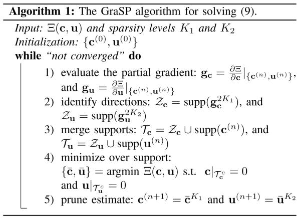
Note that (9) is a nonlinear optimization problem with a smooth, non-convex cost function and explicit sparsity constraints. For this problem, it can be shown that there exists at least one optimal solution based on the Weierstrass extreme value theorem [29], although the uniqueness of the solution can be generally difficult to establish. With respect to solving this type of problems, a number of greedy pursuit algorithms have been recently developed (e.g., [30]-[32]). These algorithms are mostly generalizations of greedy algorithms for compressive sensing with nonlinear measurements. Here, we adapt the Gradient Support Pursuit (GraSP) algorithm [32] to solve (9). GraSP is an extension of compressive sampling matching pursuit (CoSaMP) [33] or subspace pursuit (SP) [34]. It is an iterative algorithm that utilizes the gradient of the cost function to identify the candidate support of the sparse coefficients, and then solves the nonlinear optimization problem constrained to the identified support.

Specifically, the procedures of GraSP for solving (9) can be summarized in Algorithm 1. We denote the cost function in (9) as Ξ(c, u), and the solution at the nth iteration as c⁽ⁿ⁾, u⁽ⁿ⁾. At the (n+1)th iteration, we first compute the partial derivative of Ξ with respect to c and u evaluated at {c⁽ⁿ⁾, u⁽ⁿ⁾ (see Appendix A for the gradient calculation). We denote the values of these partial derivatives as ${\mathbf{g}}_{\mathbf{c}}=\frac{\partial \Xi }{\partial \mathbf{c}}{\mid }_{\{{\mathbf{c}}^{\left(n\right)},{\mathbf{u}}^{\left(n\right)}\}}$ and ${\mathbf{g}}_{\mathbf{u}}=\frac{\partial \Xi }{\partial \mathbf{u}}{\mid }_{\{{\mathbf{c}}^{\left(n\right)},{\mathbf{u}}^{\left(n\right)}\}}$.

Secondly, we identify the support sets ${\mathcal{Z}}_{\mathbf{c}}$ and ${\mathcal{Z}}_{\mathbf{u}}$ that are associated with the 2K₁ largest entries of g_c and the 2K₂ largest entries of g_u, respectively, i.e., ${\mathcal{Z}}_{\mathbf{c}}=\mathrm{supp}\left({\mathbf{g}}_{\mathbf{c}}^{2K_1}\right)$ and ${\mathcal{Z}}_{\mathbf{u}}=\mathrm{supp}\left({\mathbf{g}}_{\mathbf{u}}^{2K_2}\right)$. Intuitively, under the assumption that ${\mid \mid \widehat{\mathbf{c}}\mid \mid }_0\le K_1$ and ${\mid \mid \widehat{\mathbf{u}}\mid \mid }_0\le K_2$, minimization of Ξ(c, u) over ${\mathcal{T}}_{\mathbf{c}}$ and ${\mathcal{T}}_{\mathbf{u}}$ would lead to the most effective reduction in the cost function value.

Thirdly, we merge ${\mathcal{Z}}_{\mathbf{c}}$ with supp(c⁽ⁿ⁾) to form a combined support set ${\mathcal{T}}_{\mathbf{c}}$ for c. Similarly, we merge ${\mathcal{Z}}_{\mathbf{u}}$ with supp(u⁽ⁿ⁾ to form a combined support set ${\mathcal{T}}_{\mathbf{u}}$ for u. It is easily shown that $\mid {\mathcal{T}}_{\mathbf{c}}\mid \le 3K_1$, and $\mid {\mathcal{T}}_{\mathbf{u}}\mid \le 3K_2$. We then minimize Ξ(c, u) over ${\mathcal{T}}_{\mathbf{c}}$ and ${\mathcal{T}}_{\mathbf{u}}$. This optimization problem is a support-constrained nonlinear optimization problem, i.e.,

$$\begin{array}{cc}\hfill \underset{\mathbf{c},\mathbf{u}}{\min }& \sum _{m=1}^M{\Vert {\mathbf{d}}_m-{\mathbf{F}}_m{\Psi }_m{\Phi }_m\left({\mathbf{W}}_1^T\mathbf{c}\right){\mathbf{W}}_2^T\mathbf{u}\Vert }_2^2,\hfill \\ \hfill & \mathbf{s}.\mathbf{t}.\mathbf{c}{\mid }_{{\mathcal{T}}_{\mathbf{c}}^c}=0\text{and}\mathbf{u}{\mid }_{{\mathcal{T}}_{\mathbf{u}}^c}=0.\hfill \end{array}$$ (10)

(10) can be easily converted into an unconstrained optimization problem by variable change. More specifically, let c = E_cc_t and u = E_uu_t where ${\mathbf{c}}_t\in {ℝ}^{\mid {\mathcal{T}}_{\mathbf{c}}\mid }$ and ${\mathbf{u}}_t\in {ℝ}^{\mid {\mathcal{T}}_{\mathbf{u}}\mid }$ contain the coefficients on the support ${\mathcal{T}}_{\mathbf{c}}$ and ${\mathcal{T}}_{\mathbf{u}}$, respectively, and ${\mathbf{E}}_{\mathbf{c}}\in {ℝ}^{N\times \mid {\mathcal{T}}_{\mathbf{c}}\mid }$ and ${\mathbf{E}}_{\mathbf{u}}\in {ℝ}^{N\times \mid {\mathcal{T}}_{\mathbf{u}}\mid }$ are two submatrices of the N × N identity matrix whose columns are selected according to ${\mathcal{T}}_{\mathbf{c}}$ and ${\mathcal{T}}_{\mathbf{u}}$, respectively. The resulting unconstrained optimization problem becomes:

$$\underset{{\mathbf{c}}_t,{\mathbf{u}}_t}{\min }\sum _{m=1}^M{\Vert {\mathbf{d}}_m-{\mathbf{F}}_m{\Psi }_m{\Phi }_m\left({\mathbf{W}}_1^T{\mathbf{E}}_{\mathbf{c}}{\mathbf{c}}_t\right){\mathbf{W}}_2^T{\mathbf{E}}_{\mathbf{u}}{\mathbf{u}}_t\Vert }_2^2.$$ (11)

Note that (11) is a nonlinear least-squares problem. Since the cost function of this unconstrained optimization problem is continuous and coercive, there exists at least one optimal solution [29], although the optimal solution may not be unique. To solve this problem, a number of numerical algorithms can be used. Here, we apply the quasi-Newton limited memory Broyden-Flecher-Goldfarb-Shanno (L-BFGS) algorithm [35]. This algorithm only needs the gradient evaluation, and the Hessian matrix is approximated by the gradient information (see Appendix A for the gradient of the cost function in (11)). Note that in our case, the scaling of two variables u and c can be quite distinct. With proper scaling compensation (e.g., through a similar procedure as used in [25], [26]), it has been empirically observed that the accuracy and convergence speed of the L-BFGS algorithm can be significantly improved.

Finally, after obtaining the solution $\stackrel{‒}{\mathbf{c}}$ and $\stackrel{‒}{\mathbf{u}}$ to (10), we only keep the largest K₁ entries of c and the largest K₂ entries of u, and set other entries to zero, i.e., ${\mathbf{c}}^{(n+1)}={\stackrel{‒}{\mathbf{c}}}^{K_1}$ and ${\mathbf{u}}^{(n+1)}={\stackrel{‒}{\mathbf{u}}}^{K_2}$. The above procedure is repeated until the relative change of Ξ between two consecutive iterations is smaller than some pre-specified threshold, or the number of iterations exceeds a pre-specified maximum number of iterations.

Computationally, the algorithm is relatively efficient: at each iteration it only involves gradient evaluation, support detection and solving a support-constrained optimization problem. For the support-constrained optimization problem, its computational complexity is smaller than (7) due to the reduced number of unknowns. It has been shown in [32] that under certain theoretical conditions (generalized restricted isometry property for linear measurement model), GraSP has guaranteed performance. However, note that verifying these theoretical conditions in the context of this problem can be very difficult.

Due to the non-convex nature of the optimization problem, the solution of the GraSP is dependent on the initialization {c⁽⁰⁾, u⁽⁰⁾}. In Section III, we will discuss the initialization used in the algorithm, which is closely related to the applied data acquisition scheme. This initial condition consistently yields good empirical results, although other initializations may potentially yield better performance.

C. Estimation-theoretic bounds

We have also derived a constrained Cramér-Rao bound (CRB) to characterize the proposed estimator (8) (or (9)). The constrained CRB provides a lower bound on the covariance of any locally unbiased estimator under constraints [36], [37]. It has been widely used to characterize various constrained parameter estimation problems (e.g., [38]-[41]). Specifically, for this work, we calculate the sparsity constrained CRB [38] to analyze the benefits of incorporating the sparsity constraints into the parameter estimation problem. We can also use it as a benchmark to evaluate the performance of the proposed method.

In the rest of this section, we first derive the CRB on the estimated parameter map $\widehat{\theta }$ in the unconstrained setting,³ then extend it to consider the incorporation of the sparsity constraints, and finally we use these bounds to characterize the performance of the ML estimator or sparsity constrained ML estimator. Considering the consistency between the unconstrained and constrained case, we derive both bounds on the sparse coefficients in the transform domain.

1) Unconstrained CRB

Note that since $\widehat{\theta }={\mathbf{W}}_1^T\widehat{\mathbf{c}}$, $\mathrm{Cov}\left(\widehat{\theta }\right)$ can be written as

$$\mathrm{Cov}\left(\widehat{\theta }\right)={\mathbf{W}}_1^T\mathrm{Cov}\left(\widehat{\mathbf{c}}\right){\mathbf{W}}_1.$$ (12)

To obtain the bounds on $\mathrm{Cov}\left(\widehat{\theta }\right)$, it suffices to derive the bounds on $\mathrm{Cov}\left(\widehat{\mathbf{c}}\right)$.

Given the data model, i.e.,

$${\mathbf{d}}_m-{\mathbf{F}}_m{\Psi }_m{\Phi }_m\left({\mathbf{W}}_1^T\mathbf{c}\right){\mathbf{W}}_2^T\mathbf{u}+{\mathbf{n}}_m,$$ (13)

the unconstrained CRB on $\widehat{\mathbf{c}}$ can be written as follows [42]:

$$\mathrm{Cov}\left(\widehat{\mathbf{c}}\right)\ge \mathbf{Z},$$ (14)

where

$$\mathbf{Z}=\left[{\mathbf{E}}_N{0}_N\right]{\mathbf{J}}^{†}\left[\begin{array}{c}\hfill {\mathbf{E}}_N\hfill \\ \hfill 0_N\hfill \end{array}\right],$$ (15)

E_N is the N × N identity matrix, J is the Fisher information matrix (FIM) (see see Appendix B for a detailed derivation of the FIM) for the model in (13), and † denotes the Moore-Penrose pseudo-inverse. Substituting (14) into (12) yields the following unconstrained CRB on $\widehat{\theta }$:

$$\mathrm{Cov}\left(\widehat{\theta }\right)\ge {\mathbf{W}}_1^T{\mathbf{ZW}}_1.$$ (16)

Taking the diagonal entries of the matrices on the both sides of (16), we can obtain a lower bound for the variance of each voxel in $\widehat{\theta }$

$$\mathrm{Var}\left({\widehat{\theta }}_n\right)\ge {\left[{\mathbf{W}}_1^T{\mathbf{ZW}}_1\right]}_{n,n}.$$ (17)

Due to the large dimensionality of u and c, it is much computationally efficient to evaluate J^† in (15) using the inversion of its submatrices. Let the partitioned J be

$$\mathbf{J}=\left[\begin{array}{cc}\hfill {\mathbf{J}}_{\mathbf{c},\mathbf{c}}\hfill & \hfill {\mathbf{J}}_{\mathbf{c},\mathbf{u}}\hfill \\ \hfill {\mathbf{J}}_{\mathbf{u},\mathbf{c}}\hfill & \hfill {\mathbf{J}}_{\mathbf{u},\mathbf{u}}\hfill \end{array}\right].$$ (18)

Using the pseudo-inverse of the partitioned Hermitian matrix [43], J^† can be written as follows⁴:

$${\mathbf{J}}^{†}=\left[\begin{array}{cc}\hfill {\mathbf{J}}_{\mathbf{c},\mathbf{c}}^{†}+{\mathbf{J}}_{\mathbf{c},\mathbf{c}}^{†}{\mathbf{J}}_{\mathbf{c},\mathbf{u}}{\mathbf{V}}^{†}{\mathbf{J}}_{\mathbf{u},\mathbf{c}}{\mathbf{J}}_{\mathbf{c},\mathbf{c}}^{†}\hfill & \hfill -{\mathbf{J}}_{\mathbf{c},\mathbf{c}}^{†}{\mathbf{J}}_{\mathbf{c},\mathbf{u}}{\mathbf{V}}^{†}\hfill \\ \hfill -{\mathbf{V}}^{†}{\mathbf{J}}_{\mathbf{u},\mathbf{c}}{\mathbf{J}}_{\mathbf{c},\mathbf{c}}^{†}\hfill & \hfill {\mathbf{V}}^{†},\hfill \end{array}\right]$$ (19)

where $\mathbf{V}={\mathbf{J}}_{\mathbf{u},\mathbf{u}}-{\mathbf{J}}_{\mathbf{u},\mathbf{c}}{\mathbf{J}}_{\mathbf{c},\mathbf{c}}^{†}{\mathbf{J}}_{\mathbf{c},\mathbf{u}}$. By substituting (19) into (15), we can obtain the simplified expression for Z:

$$\mathbf{Z}=({\mathbf{J}}_{\mathbf{c},\mathbf{c}}^{†}+{\mathbf{J}}_{\mathbf{c},\mathbf{c}}^{†}{\mathbf{J}}_{\mathbf{c},\mathbf{u}}{\mathbf{V}}^{†}{\mathbf{J}}_{\mathbf{u},\mathbf{c}}{\mathbf{J}}_{\mathbf{c},\mathbf{c}}^{†}).$$ (20)

2) Constrained CRB

With the sparsity constraints on c and u, i.e.,

$${\Vert \mathbf{c}\Vert }_0\le K_1\text{and}{\Vert \mathbf{u}\Vert }_0\le K_2,$$ (21)

(assuming K₁ and K₂ are given), and the data model (13), the sparsity constrained CRB for any locally unbiased estimator $\widehat{\mathbf{c}}$ can be expressed as follows [38]:

$$\mathrm{Cov}\left(\widehat{\mathbf{c}}\right)\ge {\mathbf{Z}}_s,$$ (22)

where

$${\mathbf{Z}}_s=\left[{\mathbf{E}}_N{0}_N\right]\mathbf{A}{\left({\mathbf{A}}^T\mathbf{JA}\right)}^{†}{\mathbf{A}}^T\left[\begin{array}{c}\hfill {\mathbf{E}}_N\hfill \\ \hfill 0_N\hfill \end{array}\right],$$ (23)

$\mathbf{A}=\left[\begin{array}{cc}\hfill {\mathbf{E}}_{\mathbf{c}}\hfill & \hfill 0\hfill \\ \hfill 0\hfill & \hfill {\mathbf{E}}_{\mathbf{u}}\hfill \end{array}\right]$ E_c and E_u are two sub-matrices of E_Nwhose columns are selected based on the support of c and u, respectively. Based on (12) and (22), the constrained CRB on $\widehat{\theta }$ can be expressed as

$$\mathrm{Cov}\left(\widehat{\theta }\right)\ge {\mathbf{W}}_1^T{\mathbf{Z}}_s{\mathbf{W}}_1,$$ (24)

and the corresponding voxelwise variance bound can be expressed as:

$$\mathrm{Var}\left({\widehat{\theta }}_n\right)\ge {\left[{\mathbf{W}}_1^T{\mathbf{Z}}_s{\mathbf{W}}_1\right]}_{n,n}.$$ (25)

Similar to the unconstrained case, we can further simplify the calculation of Z_s using the block matrix pseudo-inversion. Let the partitioned A^T JA be

$${\mathbf{A}}^T\mathbf{JA}=\left[\begin{array}{cc}\hfill {\mathbf{G}}_{11}\hfill & \hfill {\mathbf{G}}_{12}\hfill \\ \hfill {\mathbf{G}}_{21}\hfill & \hfill {\mathbf{G}}_{22}\hfill \end{array}\right],$$

where ${\mathbf{G}}_{11}={\mathbf{E}}_{\mathbf{c}}^T{\mathbf{J}}_{\mathbf{cc}}{\mathbf{E}}_{\mathbf{c}}$, ${\mathbf{G}}_{12}={\mathbf{E}}_{\mathbf{c}}^T{\mathbf{J}}_{\mathbf{cu}}{\mathbf{E}}_{\mathbf{u}}$, ${\mathbf{G}}_{21}={\mathbf{G}}_{12}^T$ and ${\mathbf{G}}_{22}={\mathbf{E}}_{\mathbf{u}}^T{\mathbf{J}}_{\mathbf{uu}}{\mathbf{E}}_{\mathbf{u}}$. Again, with the pseudo-inverse of the partitioned Hermitian matrix [43], (A^T JA)^† can be expressed as

$${\left({\mathbf{A}}^T\mathbf{JA}\right)}^{†}=\left[\begin{array}{cc}\hfill {\mathbf{G}}_{11}^{†}+{\mathbf{G}}_{11}^{†}{\mathbf{G}}_{12}{\mathbf{Q}}_s^{†}{\mathbf{G}}_{21}{\mathbf{G}}_{11}^{†}\hfill & \hfill -{\mathbf{G}}_{11}^{†}{\mathbf{G}}_{12}{\mathbf{Q}}_s^{†}\hfill \\ \hfill -{\mathbf{Q}}_s^{†}{\mathbf{G}}_{21}{\mathbf{G}}_{11}^{†}\hfill & \hfill {\mathbf{Q}}_s^{†}\hfill \end{array}\right],$$ (26)

where ${\mathbf{Q}}_s={\mathbf{G}}_{22}-{\mathbf{G}}_{21}{\mathbf{G}}_{11}^{†}{\mathbf{G}}_{12}$. Substituting (26) into (23) yields the following simplified expression for Z_s:

$${\mathbf{Z}}_s={\mathbf{E}}_{\mathbf{c}}({\mathbf{G}}_{11}^{†}+{\mathbf{G}}_{11}^{†}{\mathbf{G}}_{12}{\mathbf{Q}}_s^{†}{\mathbf{G}}_{21}{\mathbf{G}}_{11}^{†}){\mathbf{E}}_{\mathbf{c}}^T,$$ (27)

where ${\mathbf{Q}}_s={\mathbf{G}}_{22}-{\mathbf{G}}_{21}{\mathbf{G}}_{11}^{†}{\mathbf{G}}_{12}$.

3) Performance Characterization

Under the assumption that there is no model mismatch in the data model (13), and that the ML estimator ${\widehat{\theta }}_{\mathrm{ML}}$ is unbiased, the unconstrained CRB can provide a lower bound on the covariance, or mean-squared-error (MSE), of ${\widehat{\theta }}_{\mathrm{ML}}$ in (7) [46]. Note that this bound can also be asymptotically achieved by the ML estimator [42], i.e., when Σ_m=1 P_m → ∞. Similarly, under the assumption that there is no model mismatch in either the data model (13) or the sparsity model (21), and that the constrained ML estimator ${\widehat{\theta }}_{\mathrm{sML}}$ is locally unbiased, (24) can also be used to characterize the covariance, or the mean-squared error (MSE), of ${\widehat{\theta }}_{\mathrm{sML}}$ in (8).

Furthermore, under no mismatch in the signal model and data model, it can be shown [36], [38] that

$${\mathbf{W}}_1^T{\mathbf{ZW}}_1\ge {\mathbf{W}}_1^T{\mathbf{Z}}_s{\mathbf{W}}_1,$$ (28)

which confirms the benefits of the sparsity constraints. In the next section, we will calculate the above bounds in a specific application to further illustrate this point.

III. Results

In this section, representative simulation results from T₂ mapping of the brain are shown to illustrate both the estimation-theoretic bounds and the empirical performance of the proposed method.

The following metrics are used to evaluate the performance of different reconstruction methods: 1) normalized error (NE) at the nth voxel:

$${\mathrm{NE}}_n=\frac{1}{{\theta }_n}\mid {\theta }_n-{\widehat{\theta }}_n\mid ,$$ (29)

where ${\widehat{\theta }}_n$ denotes the reconstructed parameter value at the nth voxel, 2) ROI normalized error (rNE):

$$\mathrm{rNE}=\frac{1}{{\theta }_{\mathrm{ROI}}}\mid {\theta }_{\mathrm{ROI}}-{\widehat{\theta }}_{\mathrm{ROI}}\mid ,$$ (30)

where θ_ROI and ${\widehat{\theta }}_{\mathrm{ROI}}$ respectively denote the averaged parameter values within the ROI from the ground truth and estimator, 3) normalized root-mean-squared-error (NRMSE) at the nth voxel:

$${\mathrm{NRMSE}}_n=\frac{1}{{\theta }_n}\sqrt{\mathbf{E}\left[{\mid {\theta }_n-{\widehat{\theta }}_n\mid }^2\right],}$$ (31)

and 4) ROI normalized root-mean-squared-error (rNRMSE) in a ROI:

$$\mathrm{rNRMSE}=\sqrt{\frac{1}{N_{\mathrm{ROI}}}\sum _{n\in \mathrm{ROI}}{\mathrm{NRMSE}}_n^2.}$$ (32)

The first two metrics are used to evaluate the accuracy for one noise realization in a simulation, whereas the last two metrics are used to evaluate the accuracy in Monte Carlo simulations.⁵

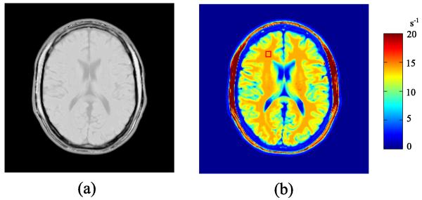
A realistic numerical brain phantom from the Brainweb database [47] was used to simulate a single-channel, multi-echo spin-echo T₂ mapping experiment. For this experiment, the contrast weighting function is φ(θ, γ_m) = exp(−T_EmR₂), where θ = R₂ is the transverse relaxation rate (i.e., the reciprocal of T₂), and γ_m = T_Em denotes the mth echo time. For the spin-echo imaging sequence, the phase distribution matrix Ψ_m can be assumed to be an identity matrix [26], for m = 1, ⋯, M. The spin density map and R₂ map of the phantom are shown in Fig. 1.

Fig. 1.

Numerical brain phantom: a) the spin density map, and b) the R₂ map (with a marked ROI in the white matter).

The imaging sequence consists of M = 16 equally spaced echoes with the first echo time T_E1 = 12.5ms and the echo spacing ΔT_E = 9.5ms. The acquisition matrix is 256 × 256, and the spatial resolution is 1 × 1 mm². We performed retrospective undersampling with a sampling pattern that acquires full k-space samples for the first echo time and sparse k-space data (with a unform random sampling pattern) for the remaining echo times. The acceleration factor (AF) is defined as $NM∕{\Sigma }_{m=1}^M$ P_m, i.e., the total number of voxels in the image sequence divided by the total number of measurements, to measure the undersampling levels. The SNR is defined as 20 log₁₀(s/σ), where s denotes the average signal intensity within a region of the gray matter in the T₂-weighted image with the longest echo time, and σ denotes the noise variance.

Simulations were performed in the following two settings. In the first setting, we used a data set that has 1) a monoexponential T₂ relaxation, and 2) ρ and R₂ maps that are sparse in the wavelet domain. Specifically, we synthesized the ρ and R₂ maps using their largest 20% wavelet coefficients with the Daubechies 4 wavelet transform and three-level decomposition. The T₂-weighted image sequence ${\left\{I_m\right(\mathbf{x}\left)\right\}}_{m=1}^M$ was then generated using the monoexponential T₂ relaxation model. This scenario is referred to as the simulation setting without model mismatch. In the second setting, we used the original brain phantom from the Brainweb database. This phantom was simulated in a way that both signal model mismatch (multiexponential relaxation caused by partial volume effect [47]) and sparsity model mismatch (the wavelet coefficients are just compressible) exist. This scenario is referred to as the simulation setting with model mismatch.

A. Without model mismatch

We evaluated the performance of the following three methods: the ML estimator in (7), the proposed estimator in (8), and an oracle estimator that assumes complete knowledge of the support of the wavelet coefficients of θ and ρ. Mathematically, the oracle estimator $\{{\widehat{\rho }}_{\mathrm{o}},{\widehat{\theta }}_{\mathrm{o}}\}$ can be defind as ${\widehat{\rho }}_{\mathrm{o}}={\mathbf{W}}_2{\widehat{\mathbf{u}}}_{\mathrm{o}}$ and ${\widehat{\theta }}_{\mathrm{o}}={\mathbf{W}}_1{\widehat{\mathbf{c}}}_{\mathrm{o}}$ with

$$\begin{array}{cc}\hfill \{{\widehat{\mathbf{c}}}_{\mathrm{o}},{\widehat{\mathbf{u}}}_{\mathrm{o}}=\arg \underset{\mathbf{c},\mathbf{u}}{\min }& \sum _{m=1}^M{\Vert {\mathbf{d}}_m-{\mathbf{F}}_m{\Psi }_m{\Phi }_m\left({\mathbf{W}}_1^T\mathbf{c}\right){\mathbf{W}}_2^T\mathbf{u}\Vert }_2^2,\hfill \\ \hfill & \mathbf{s}.\mathbf{t}.\mathbf{c}{\mid }_{{\mathcal{T}}_1^c}=0\text{and}\mathbf{u}{\mid }_{{\mathcal{T}}_2^c}=0,\hfill \end{array}$$ (33)

where ${\mathcal{T}}_1$ and ${\mathcal{T}}_2$ represent the true support sets of the wavelet coefficients of θ and ρ, respectively. Although the oracle estimator is generally impossible to implement in practice, its performance can indicate the best performance that the proposed estimator could achieve. It can be shown that the oracle estimator asymptotically achieves the constrained CRB, and that it is asymptotically unbiased (see Appendix C).

For the ML estimator, ρ was initialized with the image reconstructed from the fully sampled data at the first echo, and R₂ was initialized with zero. For the oracle estimator, u_o was initialized with the largest 0.2N wavelet coefficients of the reconstructed image from the first echo, and c_o was initialized with zero. For the proposed method, the same initializations as the oracle estimator were used. It was observed empirically that the above initializations consistently yielded good reconstruction results, although other initializations may result in further improvement. In terms of sparsity level, we set K₁ = K₂ = 0.2N, i.e., the proposed estimator knows the true sparsity level, but it does not have any knowledge of the support sets of the sparse wavelet coefficients.

To numerically determine the ML estimator and the oracle estimator, the L-BFGS algorithm was used, in which the maximum number of iterations was set to be 150 for both estimators. For the proposed estimator, we used the GraSP algorithm as described in Section II-B. Specifically, for the subproblem (11) in GraSP, we applied the L-BFGS algorithm as well, for which the maximum number of iteration was also set to be 150. With respect to the stopping criterion of GraSP, we terminated the algorithm, when either 1) the maximum iteration is larger than 20, or 2) the relative change of the cost function value between two consecutive iterations is less than 1e⁻⁴.

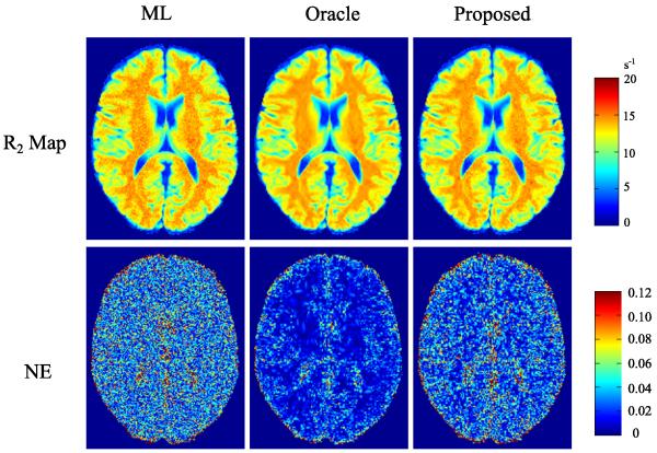
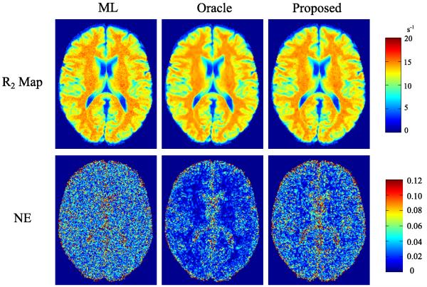
We performed reconstructions using the three methods for AF = 4 and SNR = 30 dB. The reconstructed R₂ maps and their corresponding NE are shown in Fig. 2.⁶ As can be seen qualitatively, the proposed method reduced noise corruption, comparing to the R₂ reconstructed by the ML estimator. Quantitatively, the proposed method also has better accuracy than the ML estimator that only takes advantage of the contrast-weighting signal model, although the proposed method is inferior to the oracle estimator, as expected. For a ROI in the white matter (labeled in Fig. 1), the rNEs are 2.13%, 1.17%, 1.50% for the ML, oracle, and proposed estimators, consistent with the comparison shown in Fig. 2.

Fig. 2.

Reconstructed R₂ maps and corresponding NE maps for the simulations without model mismatch, from the ML estimator, the oracle estimator, and the proposed estimator, at AF = 4 and SNR = 30 dB.

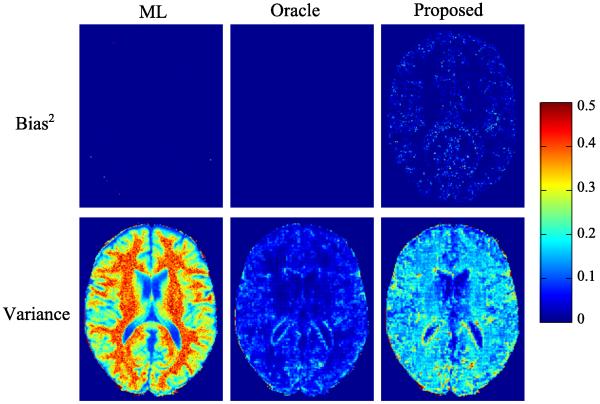
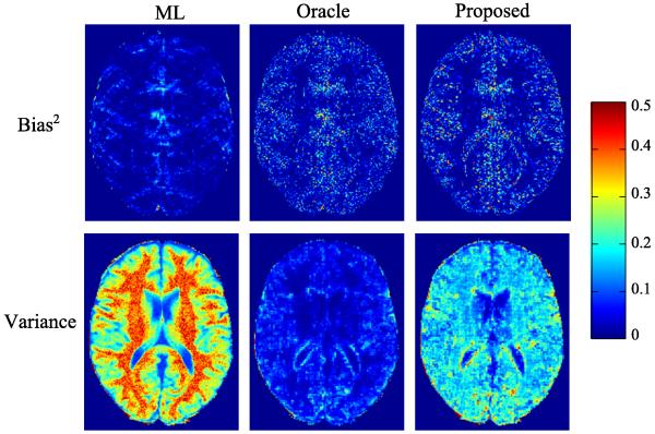
We conducted MC simulations (with 200 trials) to investigate the statistical properties of the three estimators empirically. Fig. 3 illustrates the empirical bias and variance of each estimator. The bias from the ML estimator and the oracle estimator are almost negligible, confirming that these two estimators are asymptotically unbiased in theory. The proposed estimator has larger bias than the ML. Compared to the oracle, it has also larger bias due to its error in support detection. In terms of variance, the proposed estimator has much smaller values than the ML estimator, due to the sparsity constraints. Furthermore, we see that for all three estimators, their variances are much larger than their corresponding squared biases, which implies the MSE is dominated by the variance component in the current simulation setting.

Fig. 3.

Squared bias and variance of the ML estimator, the oracle estimator, and the proposed estimator at AF = 4 and SNR = 30 dB for the simulations without model mismatch.

In addition to the above MC study, we calculated the estimation-theoretic bounds using (17) and (25) to analyze the benefits of sparsity constraints. The two bounds also inform the performance limits of the ML estimator and the proposed estimator in the absence of modeling errors. We also calculated the NRMSE of the three estimators from the MC study. To compare the performance bounds with the NRMSE at the right scale, we use the following normalized CRB and CCRB:

$$\begin{array}{cc}\hfill {\mathbf{nCRB}}_n=& \frac{1}{{\theta }_n}\sqrt{{\left[{\mathbf{W}}_1^T{\mathbf{ZW}}_1\right]}_{n,n}},\hfill \\ \hfill {\mathbf{nCCRB}}_n=& \frac{1}{{\theta }_n}\sqrt{{\left[{\mathbf{W}}_1^T{\mathbf{Z}}_s{\mathbf{W}}_1\right]}_{n,n}}.\hfill \end{array}$$ (34)

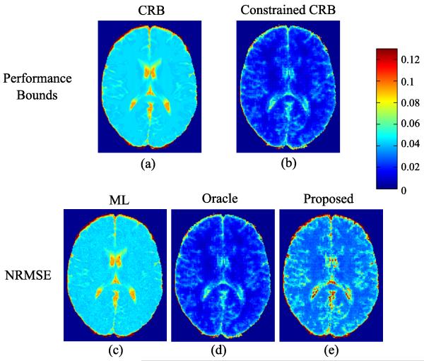
Fig. 4 shows the performance bounds and NRMSE maps. As can be seen, the normalized CRB predicts the NRMSE of the ML estimator well, while the normalized CCRB accurately captures the NRMSE of the oracle estimator. Both theoretical results and empirical study clearly demonstrate the benefits of incorporating the sparsity constraints. Take a square ROI in the white matter (labeled in Fig. 1) for example. From the normalized CRB and CCRB maps, it can be seen that by incorporating the sparsity constraints with K₁ = K₂ = 0.2N, the reconstruction error at best decreases from 4.17% to 1.27%. As one practical estimator, the proposed method attains the reconstruction error at around 2.78%, which is better than the ML estimator.

Fig. 4.

Estimation-theoretic bounds and NRMSE maps for the simulation setting without model mismatch: a) normalized CRB map, b) normalized constrained CRB map, c)-e) NRMSE maps of the ML, oracle, and proposed estimators.

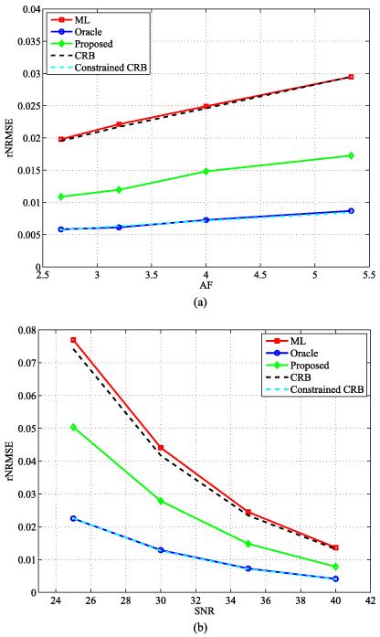
We studied the performance bounds and empirical performance of the three estimators at different undersampling sampling levels. The MC simulations were performed for AF = 2.67, 3.2, 4, and 5.33, all with SNR = 35 dB. The rNRMSE (with the ROI labeled in Fig. 1) was computed. We also calculated the performance bounds at the above undersampling levels. Fig. 5(a) shows the plot of the rNRMSE and the normalized performance bounds with respect to AF. As expected, both performance bounds and the empirical performance of the three estimators become worse when AF increases. Consistent with the previous results, the two performance bounds well predicts the empirical performance of the ML and oracle estimators, respectively. The proposed estimator improves over the ML estimator at all AFs. Note that the rNRMSE of the proposed estimator at AF = 5.33 is smaller than that of the ML estimator at AF = 2.67, i.e., the proposed estimator achieves even better performance than the ML estimator when it only uses half amount of k-space data as the ML estimator.

Fig. 5.

The rNRMSE and estimation-theoretic bounds with respect to different AF or SNR: a) rNRMSE and normalized performance bounds versus AF, b) rNRMSE and normalized performance bounds versus SNR.

We also studied the performance bounds and empirical performance of the three estimators at different SNR levels, i.e., SNR = 25, 30, 35, and 40 dB, all with AF = 4. The plot of rNRMSE (with the same ROI) and the normalized performance bounds with respect to SNR are shown in Fig. 5(b). It can be seen that the proposed estimator has improved noise robustness over the ML estimator, both theoretically and empirically, at all tested SNR levels. Note that the proposed estimator achieves a similar rNRMSE at SNR = 35 dB to what the ML estimator does at SNR = 40 dB.

B. With model mismatch

We also performed simulations to study the performance of the proposed method with model mismatch. In this simulation setting, the proposed estimator and the oracle will be affected by the modeling errors from both the monoexponential model and sparse approximation, while the ML estimator is only influenced by the monoexponential model mismatch.

For the proposed method, we empirically set the sparsity level K₁ = K₂ = 0.2N, which is the same as the previous simulations. For the oracle estimator, we set ${\mathcal{T}}_1$ and ${\mathcal{T}}_2$ as two support sets that contain the largest 0.2N wavelet coefficients of ρ andθ, respectively. Furthermore, for the numerical solvers of three estimators, we followed the same implementation as described for the simulations without model mismatch.

We performed reconstructions using the three methods under AF = 4 and SNR = 30 dB. The reconstructed R₂ maps, along with the corresponding NE maps, are shown in Fig. 6. This figure demonstrates the improvement of the oracle and the proposed estimator over the ML estimator. For the ROI in the white matter, the rNEs are 2.41%, 1.47%, and 1.71% for the ML, oracle, and the proposed estimator.

Fig. 6.

Reconstructed R₂ maps for the simulations with model mismatch, from the ML estimator, oracle estimator, and proposed estimator, under AF = 4 and SNR = 30 dB.

Fig. 7 shows the bias-variance analysis of the three estimators from the MC simulations (with 200 trials) under AF = 4 and SNR = 30 dB, and Fig. 8 shows the corresponding NRMSE maps. With the sparsity constraints, the oracle and proposed estimators have significantly reduced variance and NRMSE than the ML estimator. Compared to the case without modeling error, the three estimators exhibit similar level of variance. However, in terms of biases, the three estimators all have increased values. It is worth noting that the squared bias of the ML estimator exhibits an aliasing-like pattern, which is different from those of the oracle and the proposed estimator. This is due to the different modeling errors that they have.

Fig. 7.

Squared bias and variance for the ML estimator, oracle estimator, and the proposed estimator from the simulations with model mismatch.

Fig. 8.

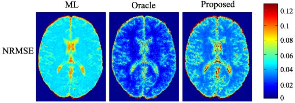
NRMSE maps for the ML estimator, oracle estimator, and the proposed estimator from the simulations with model mismatch.

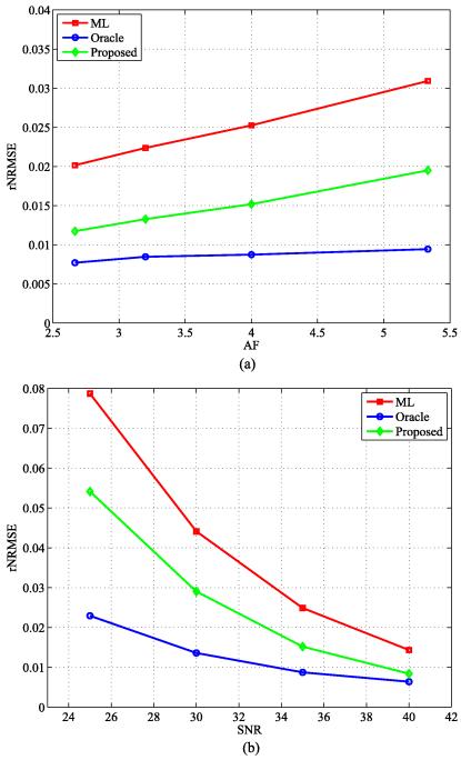
We again performed MC simulations to evaluate the three estimators at different undersampling levels, i.e., AF = 2.67, 3.2, 4, and 5.33, with SNR = 35 dB. We also performed the MC simulations at different noise levels, i.e., SNR = 25, 30, 35, and 40 dB, with AF = 4. The plot of the rNRMSE (with the same ROI) with respect to AF, as well as rNRMSE with respect to SNR, is shown in Fig. 9 (a) and (b), respectively. This figure further demonstrates that the proposed method improves over the ML estimator even in the presence of modeling errors, at different undersampling levels or noise levels.

Fig. 9.

The rNRMSE plot at different AF and SNR for the simulations with model mismatch: a) the rNRMSE versus AF, and b) the rNRMSE versus SNR.

IV. Discussion

The proposed method imposes sparsity constraints on both the relaxation parameter map θ and the proton density map ρ, which extends our early work [27] that only enforces the sparsity constraint on θ. Although ρ is assumed to be the nuisance parameter, we observed that imposing the sparsity constraint on ρ slightly improved the reconstruction accuracy for θ. Furthermore, with the additional sparsity constraint, the computation and memory usage for calculating the constrained CRB is significantly reduced, since the matrices in (27) have much smaller sizes.

The proposed estimator needs to specify the sparsity levels K₁ and K₂ in (9), which will impact the sparse approximation error and noise amplification of the resulting parameter maps. It is also directly related to the trade-off between bias and variance of the proposed estimator. If K₁ and K₂ are too small, severe sparse approximation error can incur significant bias that dominates MSE. On the contrary, if K₁ and K₂ are too large, significant variance due to noise amplification can diminish the benefit of the sparsity constraints and the performance of the proposed method can be very close to that of the ML estimator. In the paper, we manually set K₁ and K₂, with the reference of the underlying ground truth, to balance the bias and variance of the proposed estimator. For some specific applications (e.g., T₂ mapping for brains), the level of sparse approximation error might be roughly known, which could assist the sparsity level selection. Generally, choosing sparsity levels in a principled way, in the absence of the ground truth, is still an open problem, which requires further systematic study.

The parametric signal model that assumes a monoexponential relaxation process has been used in the proposed method. In some practical applications, a multi-exponential signal model may be more accurate [48]-[50]. The proposed method, including the algorithm and performance bounds, can be generalized to multiexponential signal models, although the optimization problem will be more difficult. Furthermore, in some specific applications (e.g., variable flip angle T₁ mapping), it would be beneficial to take into account of imperfections in data acquisition [51], such as B₁ field inhomogeneity. These imperfections can also be incorporated into the signal model used in the proposed method, although the estimation problem could have increased noise sensitivity due to the increased number of unknowns.

The proposed method predetermines the phase distribution ${\left\{{\Psi }_m\right\}}_{m=1}^M$ and incorporates it into the signal model in (3). In many applications, the phase distribution can be accurately pre-estimated from auxiliary data. This way of formulating the problem simplifies the algorithm and calculation of the performance bounds. However, note that the proposed method can be generalized such that the phase distribution can be treated as unknown. One straightforward extension is to reformulate the problem with the separate real and imaginary components of ρ, and modify the algorithm and performance bound calculation accordingly. Alternatively, we can also directly deal with complex ρ in the estimation problem. Note that this extension requires careful complexification in solving the nonlinear least-squares problem in (11) (see [52] and references therein) and calculating estimation-theoretic bounds [53], [54].

The propose method imposes explicit sparsity constraints through the ℓ₀ quasi-norm. Alternatively, sparsity constraints can also be enforced using other penalty functions (such as the ℓ₁, or total-variation regularizations). With those sparsity constraints, the reconstruction problem can be formulated as a penalized maximum likelihood (PML) estimation problem. In [55], we have presented an investigation along this direction. Preliminary results demonstrate that these two different methods imposing sparsity constraints can lead to distinct bias-variance trade-off under different SNR regimes. Systematic study of the difference will be presented in the future work.

The accuracy of the GraSP algorithm for the proposed method depends critically on the accuracy of solving the nonconvex subproblem (11), which involves the multiplicative coupling of two optimization variables u and c. A poor solution from (11) can lead the GraSP algorithm to an inaccurate reconstruction. However, in our case, we have empirically observed that with a proper initialization and scaling compensation, the L-BFGS algorithm can converge to a reasonable stationary point, leading to a fairly accurate final reconstruction.

Although the proposed method improves over the ML estimation, there is still a relatively large gap between its empirical performance and the constrained CRB when SNR is low or the undersampling level is high. There are ways to potentially improve the proposed method, and drive its performance closer to the constrainted CRB. One possibility is to use a solution algorithm of better accuracy than the current GraSP algorithm. Viable candidates to be studied include [30], [31]). Another possibility is to use stronger sparsity constraints (e.g., the structured sparsity) on u and c for the estimation problem. For example, the tree structured sparsity constraints [56] on the wavelet coefficients could be incorporated into (9). Note that following a similar procedure in [56], the GraSP algorithm could be also extended to solve the resulting new constrained estimation problem.

Regarding the computational efficiency, it takes about 16 minutes to run the GraSP algorithm for the data set in Section III on a workstation with a 3.47GHz dual-hex-core Intel Xeon processor X5690, 96 GB RAM, Linux system and Matlab R2012a. Since, at each iteration, the running time for the gradient evaluation and support operation is almost negligible compared to solving the subproblem (11) by the the L-BFGS algorithm, the overall efficiency of the algorithm may be considerably improved by using faster numerical solvers for (11). The majorization-minimization (MM) based algorithms [57] might be a viable alternative, since these algorithms can decompose the original optimization problem into a series of simplified problem, which may lead to acceleration. Also, note that (11) is a separable nonlinear least-squares problem (i.e., when c_t is fixed, it becomes a linear least-squares problem with respect to u_t), thus the variable projection algorithm [58] can be utilized to solve (11), which might result in better convergence.

In this work, the theoretical analysis with the sparsity constrained CRB relies on the assumption in (21). Note that if the coefficients c and u are only approximately sparse (or compressible), sparsity constrained CRB is not applicable in theory, although it may still provide some useful insights in practice. In this case, different types of performance bounds may be needed, depending on the class of signal models considered. For example, if we assume certain compressible prior distributions [59] on c and u, the parameter estimation problem can be posed within the Bayesian estimation framework and the Bayesian CRB [60]-[62] could be used for performance characterization. Systematic investigation of these extensions will be carried out in the future work.

For the sake of simplicity, we used the orthonormal wavelet transform as an example to illustrate the performance of our proposed method. But note that both the algorithm and theoretical analysis can be extended to incorporate other types of sparse representations, such as overcomplete sparsifying transforms (e.g., [63]) or learned dictionaries (e.g., [64], [65]), which may lead to better performance. Also note that if overcomplete sparsifying transforms are used for θ and ρ, although (8) is no longer equivalent to (9), the synthesis form of the formulation (9) still applies. Furthermore, extension to analysis-type sparsifying transforms would also be an interesting problem for future investigation. Some preliminary work has been done using the finite difference within the ℓ₁-PML formulation [55], and it might also be interesting to explore the extension to the ℓ₀ constrained formulation.

It is also worthwhile to note that the proposed method is not restricted to the sampling scheme described in this paper. It allows for flexible acquisition design in specific application scenarios, although the initialization and phase estimation schemes need to be changed accordingly. The estimation-theoretical bounds presented in the paper can also provide useful tools to assist experimental design (i.e., selection of sampling patterns or sequence parameters).

In this work, we focus on presenting the algorithmic and theoretical contributions of our work, and demonstrate the performance of the proposed method using simulations. Systematic experimental study are needed to further evaluate the practical utility of the proposed method. In this case, some practical issues also need to be taken into account, such as the generalization to multichannel acquisitions [66] and compensation of effects from sequence imperfection [67].

V. Conclusion

This paper presented a new method to accelerate MR parameter mapping with sparse sampling. It directly reconstructs parameter maps from highly undersampled, noisy k-space data, utilizing an explicit signal model while imposing sparsity constraint on the parameter values. An efficient greedy-pursuit algorithm was presented to solve the underlying optimization problem. The properties and performance of the proposed method were analyzed theoretically using estimation-theoretic bounds and also illustrated using a T₂ mapping application example with computer simulations. We expect that the proposed method will prove useful for various MR parameter mapping applications.

Appendix A

Gradients Calculation

This appendix presents a detailed derivation for the gradients $\frac{\partial \Xi }{\partial \mathbf{c}}$ and $\frac{\partial \Xi }{\partial \mathbf{u}}$, and also the gradient for the cost function in (11). First, we derive $\frac{\partial \Xi }{\partial \mathbf{c}}$ and $\frac{\partial \Xi }{\partial \mathbf{u}}$. Recall that Ξ(c, u) denotes the cost function in (9). For simplicity, we introduce an auxiliary variable ${\tilde{\mathbf{I}}}_m$ defined as

$${\tilde{\mathbf{I}}}_m={\Phi }_m\left(\theta \right)\rho .$$ (35)

Using the chain rule of the derivative, we have

$$\begin{array}{cc}\hfill \frac{\partial \Xi }{\partial \mathbf{c}}=& \sum _{m=1}^M{\left(\frac{\partial \theta }{\partial \mathbf{c}}\right)}^T{\left(\frac{\partial {\tilde{\mathbf{I}}}_m}{\partial \theta }\right)}^T\frac{\partial \Xi }{\partial {\tilde{\mathbf{I}}}_m}\hfill \\ \hfill =& \sum _{m=1}^M{\mathbf{W}}_1\frac{\partial {\tilde{\mathbf{I}}}_m}{\partial \theta }{\mathbf{q}}_m\hfill \\ \hfill \frac{\partial \Xi }{\partial \mathbf{u}}=& \sum _{m=1}^M{\left(\frac{\partial \rho }{\partial \mathbf{u}}\right)}^T{\left(\frac{\partial {\tilde{\mathbf{I}}}_m}{\partial \rho }\right)}^T\frac{\partial \Xi }{\partial {\tilde{\mathbf{I}}}_m}\hfill \\ \hfill =& \sum _{m=1}^M{\mathbf{W}}_2{\Phi }_m\left({\mathbf{W}}_1^T\mathbf{c}\right){\mathbf{q}}_m\hfill \end{array}$$ (36)

where $\frac{\partial {\tilde{\mathbf{I}}}_m}{\partial \theta }$ is a diagonal matrix with ${\left[\frac{\partial {\tilde{\mathbf{I}}}_m}{\partial \theta }\right]}_{n,n}={\rho }_n\frac{\partial \varphi }{\partial \theta }{\mid }_{\{{\theta }_n,{\gamma }_m\}}$, and

$${\mathbf{q}}_m=\mathbf{Re}\left\{{\left({\mathbf{F}}_m{\Psi }_m\right)}^H\left[{\mathbf{F}}_m{\Psi }_m{\tilde{\mathbf{I}}}_m\right]\right\}.$$ (37)

We then derive the gradient for (11). Denoting the cost function value of (11) by $\tilde{\Xi }$, its derivative with respect to c_t and u_t can be written as

$$\begin{array}{cc}\hfill \frac{\partial \tilde{\Xi }}{\partial {\mathbf{c}}_t}=& {\left(\frac{\partial \mathbf{c}}{\partial {\mathbf{c}}_t}\right)}^T\frac{\partial \tilde{\Xi }}{\partial \mathbf{c}}\hfill \\ \hfill =& \sum _{m=1}^M{\widehat{\mathbf{E}}}^T{\mathbf{W}}_1\frac{\partial {\tilde{\mathbf{I}}}_m}{\partial \theta }{\mathbf{q}}_m,\hfill \\ \hfill \frac{\partial \tilde{\Xi }}{\partial {\mathbf{u}}_t}=& {\left(\frac{\partial \mathbf{u}}{\partial {\mathbf{u}}_t}\right)}^T\frac{\partial \tilde{\Xi }}{\partial \mathbf{u}}\hfill \\ \hfill =& \sum _{m=1}^M{\tilde{\mathbf{E}}}^T{\mathbf{W}}_2{\Phi }_m\left({\mathbf{W}}_1^T\mathbf{c}\right){\mathbf{q}}_m.\hfill \end{array}$$ (38)

Appendix B

FIM for the data model (13)

In this appendix, we derive the FIM for the data model (13). Based on the definition of FIM [42], the partitioned FIM is formed as follows:

$$\begin{array}{cc}\hfill \mathbf{J}=& \left[\begin{array}{cc}\hfill {\mathbf{J}}_{\mathbf{c},\mathbf{c}}\hfill & \hfill {\mathbf{J}}_{\mathbf{c},\mathbf{u}}\hfill \\ \hfill {\mathbf{J}}_{\mathbf{u},\mathbf{c}}\hfill & \hfill {\mathbf{J}}_{\mathbf{u},\mathbf{u}}\hfill \end{array}\right]\hfill \\ \hfill =& -\left[\begin{array}{cc}\hfill \mathbf{E}\left[\frac{{\partial }^2\ln p(\mathbf{d};\mathbf{u},\mathbf{c})}{\partial {\mathbf{c}}^2}\right]\hfill & \hfill \mathbf{E}\left[\frac{{\partial }^2\ln p(\mathbf{d};\mathbf{u},\mathbf{c})}{\partial \mathbf{u}\partial \mathbf{c}}\right]\hfill \\ \hfill \mathbf{E}\left[\frac{{\partial }^2\ln p(\mathbf{d};\mathbf{u},\mathbf{c})}{\partial \mathbf{c}\partial \mathbf{u}}\right]\hfill & \hfill \mathbf{E}\left[\frac{{\partial }^2\ln p(\mathbf{d};\mathbf{u},\mathbf{c})}{\partial {\mathbf{u}}^2}\right]\hfill \end{array}\right],\hfill \end{array}$$ (39)

where $\mathbf{d}={[{\mathbf{d}}_1^H,\cdots ,{\mathbf{d}}_M^H]}^H$. In the following, we derive the expression for each submatrix of J.

Assuming n_m is complex white Gaussian noise, i.e., n_m ~ N(0, σ²), the log-likelihood function ln p (d; u, c) can be expressed as

$$\begin{array}{cc}\hfill \ln p(\mathbf{d};\mathbf{u},\mathbf{c})=& \sum _{m=1}^M\ln p({\mathbf{d}}_m;\mathbf{u},\mathbf{c})\hfill \\ \hfill =& -\frac{1}{{\sigma }^2}\sum _{m=1}^M{\Vert {\mathbf{F}}_m{\Psi }_m{\Phi }_m\left({\mathbf{W}}_1^T\mathbf{c}\right){\mathbf{W}}_2^T\mathbf{u}-{\mathbf{d}}_m\Vert }_2^2\hfill \\ \hfill & -(\ln \pi +\ln {\sigma }^2)\sum _{m=1}^M{P}_m.\hfill \end{array}$$ (40)

The first-order derivative of ln p(d; u, c) with respect to ρ and c can be expressed as:

$$\begin{array}{cc}\hfill & \frac{\partial \ln p(\mathbf{d};\mathbf{u},\mathbf{c})}{\partial \mathbf{u}}=-\frac{2}{{\sigma }^2}\sum _{m=1}^M{\left(\frac{\partial {\tilde{\mathbf{I}}}_m}{\partial \mathbf{u}}\right)}^T{\mathbf{q}}_m,\hfill \\ \hfill & \frac{\partial \ln p(\mathbf{d};\mathbf{u},\mathbf{c})}{\partial \mathbf{c}}=-\frac{2}{{\sigma }^2}\sum _{m=1}^M{\left(\frac{\partial {\tilde{\mathbf{I}}}_m}{\partial \mathbf{c}}\right)}^T{\mathbf{q}}_m,\hfill \end{array}$$ (41)

where

$$\begin{array}{cc}\hfill & \frac{\partial {\tilde{\mathbf{I}}}_m}{\partial \mathbf{u}}=\frac{\partial {\tilde{\mathbf{I}}}_m}{\partial \rho }\frac{\partial \rho }{\partial \mathbf{u}}={\Phi }_m\left({\mathbf{W}}_1^T\mathbf{c}\right){\mathbf{W}}_2^T\in {ℝ}^{N\times N},\hfill \\ \hfill & \frac{\partial {\tilde{\mathbf{I}}}_m}{\partial \mathbf{u}}=\frac{\partial {\tilde{\mathbf{I}}}_m}{\partial \theta }\frac{\partial \theta }{\partial \mathbf{c}}=\frac{\partial {\tilde{\mathbf{I}}}_m}{\partial \theta }{\mathbf{W}}_1^T\in {ℝ}^{N\times N}.\hfill \end{array}$$ (42)

and also recall that q_m is defined in (37).

Taking the second-order derivatives yields

$$\begin{array}{cc}\hfill \frac{{\partial }^2\ln p(\mathbf{d};\mathbf{u},\mathbf{c})}{\partial {\mathbf{u}}^2}=& -\frac{2}{{\sigma }^2}\sum _{m=1}^M{\left(\frac{\partial {\tilde{\mathbf{I}}}_m}{\partial \mathbf{u}}\right)}^T\mathrm{Re}\left\{{\mathbf{G}}_m\right\}\frac{\partial {\tilde{\mathbf{I}}}_m}{\partial \mathbf{u}},\hfill \\ \hfill \frac{{\partial }^2\ln p(\mathbf{d};\mathbf{u},\mathbf{c})}{\partial \mathbf{u}\partial \mathbf{c}}=& -\frac{2}{{\sigma }^2}\sum _{m=1}^M{\left(\frac{\partial {\tilde{\mathbf{I}}}_m}{\partial \mathbf{c}}\right)}^T\mathrm{Re}\left\{{\mathbf{G}}_m\right\}\frac{\partial {\tilde{\mathbf{I}}}_m}{\partial \mathbf{u}}\hfill \\ \hfill & -\frac{2}{{\sigma }^2}\sum _{m=1}^M{\mathbf{W}}_1\text{Diag}\left\{{\mathbf{q}}_m\right\}{\Lambda }_m{\mathbf{W}}_2^T,\hfill \\ \hfill \frac{{\partial }^2\ln p(\mathbf{d};\mathbf{u},\mathbf{c})}{\partial \mathbf{c}\partial \mathbf{u}}=& -\frac{2}{{\sigma }^2}\sum _{m=1}^M{\left(\frac{\partial {\tilde{\mathbf{I}}}_m}{\partial \mathbf{u}}\right)}^T\mathrm{Re}\left\{{\mathbf{G}}_m\right\}\frac{\partial {\tilde{\mathbf{I}}}_m}{\partial \mathbf{c}}\hfill \\ \hfill & -\frac{2}{{\sigma }^2}\sum _{m=1}^M{\mathbf{W}}_2\text{Diag}\left\{{\mathbf{q}}_m\right\}{\Lambda }_m{\mathbf{W}}_1^T,\hfill \\ \hfill \frac{{\partial }^2\ln p(\mathbf{d};\mathbf{u},\mathbf{c})}{\partial {\mathbf{u}}^2}=& -\frac{2}{{\sigma }^2}\sum _{m=1}^M{\left(\frac{\partial {\tilde{\mathbf{I}}}_m}{\partial \mathbf{u}}\right)}^T\mathrm{Re}\left\{{\mathbf{G}}_m\right\}\frac{\partial {\tilde{\mathbf{I}}}_m}{\partial \mathbf{c}}\hfill \\ \hfill & -\frac{2}{{\sigma }^2}\sum _{m=1}^M{\mathbf{W}}_1\text{Diag}\left\{{\mathbf{q}}_m\right\}{\mathbf{H}}_m{\mathbf{W}}_1^T.\hfill \end{array}$$ (43)

where ${\mathbf{G}}_m={\left({\mathbf{F}}_m{\Psi }_m\right)}^H{\mathbf{F}}_m,{\Psi }_m,{\Lambda }_m$ is a diagonal matrix with ${\left[{\Lambda }_m\right]}_{n,n}=\frac{\partial \varphi }{\partial \theta }{\mid }_{({\theta }_n,{\gamma }_m)}$, H_m is a diagonal matrix with ${\left[{\mathbf{H}}_m\right]}_{n,n}={\rho }_n\frac{{\partial }^2\varphi }{\partial {\theta }^2}{\mid }_{({\theta }_n,{\gamma }_m)}$, and Diag {a} converts a vector a into a diagonal matrix such that [Diag {a}]_n,n = a_n.

Evaluating the expectation of the expressions in (43) with respect to n_m yields

$$\begin{array}{cc}\hfill & \mathbf{E}\left[\frac{{\partial }^2\ln p(\mathbf{d};\mathbf{u},\mathbf{c})}{\partial {\mathbf{u}}^2}\right]=-\frac{2}{{\sigma }^2}\sum _{m=1}^M{\left(\frac{\partial {\tilde{\mathbf{I}}}_m}{\partial \mathbf{u}}\right)}^T\mathrm{Re}\left\{{\mathbf{G}}_m\right\}\frac{\partial {\tilde{\mathbf{I}}}_m}{\partial \mathbf{u}},\hfill \\ \hfill & \mathbf{E}\left[\frac{{\partial }^2\ln p(\mathbf{d};\mathbf{u},\mathbf{c})}{\partial \mathbf{c}\partial \mathbf{u}}\right]=-\frac{2}{{\sigma }^2}\sum _{m=1}^M{\left(\frac{\partial {\tilde{\mathbf{I}}}_m}{\partial \mathbf{u}}\right)}^T\mathrm{Re}\left\{{\mathbf{G}}_m\right\}\frac{\partial {\tilde{\mathbf{I}}}_m}{\partial \mathbf{c}},\hfill \\ \hfill & \mathbf{E}\left[\frac{{\partial }^2\ln p(\mathbf{d};\mathbf{u},\mathbf{c})}{\partial \mathbf{u}\partial \mathbf{c}}\right]=-\frac{2}{{\sigma }^2}\sum _{m=1}^M{\left(\frac{\partial {\tilde{\mathbf{I}}}_m}{\partial \mathbf{c}}\right)}^T\mathrm{Re}\left\{{\mathbf{G}}_m\right\}\frac{\partial {\tilde{\mathbf{I}}}_m}{\partial \mathbf{u}},\hfill \\ \hfill & \mathbf{E}\left[\frac{{\partial }^2\ln p(\mathbf{d};\mathbf{u},\mathbf{c})}{\partial {\mathbf{u}}^2}\right]=-\frac{2}{{\sigma }^2}\sum _{m=1}^M{\left(\frac{\partial {\tilde{\mathbf{I}}}_m}{\partial \mathbf{c}}\right)}^T\mathrm{Re}\left\{{\mathbf{G}}_m\right\}\frac{\partial {\tilde{\mathbf{I}}}_m}{\partial \mathbf{c}}.\hfill \end{array}$$ (44)

In obtaining (44), we use the fact that

$$\mathbf{E}\left[{\mathbf{q}}_m\right]=0,$$ (45)

based on the assumption that n_m is white Gaussian noise.

Appendix C

Asymptotic Properties of The Oracle Estimator

In this appendix, we establish the following asymptotic properties for the oracle estimator in (33).

Theorem 1. Assuming that both the data model (13) and sparsity model (21) hold, and that n_m is complex white Gaussian noise, the oracle estimator {${\widehat{\mathbf{u}}}_o$, ${\widehat{\mathbf{c}}}_o$} in (33) is asymptotically unbiased. Furthermore, the covariance of {${\widehat{\mathbf{u}}}_o$, ${\widehat{\mathbf{c}}}_o$} also asymptotically achieves the constrained CRB, i.e., A(A^TJA)^†A^T, where $\mathbf{A}=\left[\begin{array}{cc}\hfill {\mathbf{E}}_{\mathbf{c}}\hfill & \hfill 0\hfill \\ \hfill 0\hfill & \hfill {\mathbf{E}}_{\mathbf{u}}\hfill \end{array}\right]$ is defined in (23).

Proof: First, note that the oracle estimator in (33) can be determined by solving the following unconstrained optimization problem, i.e.,

$$\underset{{\mathbf{u}}_s,{\mathbf{c}}_s}{\min }\sum _{m=1}^M{\Vert {\mathbf{d}}_m-{\mathbf{F}}_m{\Psi }_m{\Phi }_m\left({\mathbf{W}}_1^T{\mathbf{E}}_{\mathbf{c}}{\mathbf{c}}_s\right){\mathbf{W}}_2^T{\mathbf{E}}_{\mathbf{u}}{\mathbf{u}}_s\Vert }_2^2,$$ (46)

through variable change u = E_uu_s and c = E_cc_s. The optimal solution of (46), {${\widehat{\mathbf{u}}}_s$, ${\widehat{\mathbf{c}}}_s$}, is the ML estimator with the data model:

$${\mathbf{d}}_m={\mathbf{F}}_m{\Psi }_m{\Phi }_m\left({\mathbf{W}}_1^T{\mathbf{E}}_{\mathbf{c}}{\mathbf{c}}_s\right){\mathbf{W}}_2^T{\mathbf{E}}_{\mathbf{u}}{\mathbf{u}}_s+{\mathbf{n}}_m.$$ (47)

Based on the invariance property of the ML estimation (Theorem 7.4 in [42]), the oracle estimator, given by

$$\left[\begin{array}{c}\hfill {\widehat{\mathbf{u}}}_o\hfill \\ \hfill {\widehat{\mathbf{c}}}_o\hfill \end{array}\right]=\mathbf{A}\left[\begin{array}{c}\hfill {\widehat{\mathbf{u}}}_s\hfill \\ \hfill {\widehat{\mathbf{c}}}_s\hfill \end{array}\right],$$ (48)

is the ML estimator of {u, c} for the model (13) and (21), and thus it is asymptotically unbiased.

Furthermore, it is known that the ML estimator {${\widehat{\mathbf{u}}}_s$, ${\widehat{\mathbf{c}}}_s$} asymptotically achieves the CRB [42], i.e.,

$$\mathrm{Cov}\left(\left[\begin{array}{c}\hfill {\widehat{\mathbf{u}}}_s\hfill \\ \hfill {\widehat{\mathbf{c}}}_s\hfill \end{array}\right]\right)\underset{=}{a}{\mathbf{J}}_s^{†}$$ (49)

where J_s is the FIM for the data model (47), defined by

$${\mathbf{J}}_s=\mathbf{E}\left[\left(\frac{\partial \ln p(\mathbf{d};{\mathbf{u}}_s,{\mathbf{c}}_s)}{\partial {[{\mathbf{u}}_s^T,{\mathbf{c}}_s^T]}^T}\right){\left(\frac{\partial \ln p(\mathbf{d};{\mathbf{u}}_s,{\mathbf{c}}_s)}{\partial {[{\mathbf{u}}_s^T,{\mathbf{c}}_s^T]}^T}\right)}^T\right],$$ (50)

which can be rewritten as

$$\begin{array}{cc}\hfill {\mathbf{J}}_s=& \mathbf{E}\left[\left({\mathbf{A}}^T\frac{\partial \ln p(\mathbf{d};\mathbf{u},\mathbf{c})}{\partial {[{\mathbf{u}}^T,{\mathbf{c}}^T]}^T}\right){\left({\mathbf{A}}^T\frac{\partial \ln p(\mathbf{d};\mathbf{u},\mathbf{c})}{\partial {[{\mathbf{u}}^T,{\mathbf{c}}^T]}^T}\right)}^T\right]\hfill \\ \hfill =& {\mathbf{A}}^T\mathbf{E}\left[\left(\frac{\partial \ln p(\mathbf{d};\mathbf{u},\mathbf{c})}{\partial {[{\mathbf{u}}^T,{\mathbf{c}}^T]}^T}\right){\left(\frac{\partial \ln p(\mathbf{d};\mathbf{u},\mathbf{c})}{\partial {[{\mathbf{u}}^T,{\mathbf{c}}^T]}^T}\right)}^T\right]\mathbf{A}\hfill \\ \hfill =& {\mathbf{A}}^T\mathbf{JA}.\hfill \end{array}$$ (51)

Finally, taking the covariance on the both sides of (48) yields

$$\begin{array}{cc}\hfill \mathrm{Cov}\left(\left[\begin{array}{c}\hfill {\widehat{\mathbf{u}}}_o\hfill \\ \hfill {\widehat{\mathbf{c}}}_o\hfill \end{array}\right]\right)=& \mathbf{A}\mathrm{Cov}\left(\left[\begin{array}{c}\hfill {\widehat{\mathbf{u}}}_s\hfill \\ \hfill {\widehat{\mathbf{c}}}_s\hfill \end{array}\right]\right){\mathbf{A}}^T\hfill \\ \hfill \underset{=}{a}& \mathbf{A}{\left({\mathbf{AJA}}^T\right)}^{†}{\mathbf{A}}^T,\hfill \end{array}$$ (52)

which establishes the second half of the theorem.

References

- [1].Margaret Cheng H-L, Stikov N, Ghugre NR, Wright GA. Practical medical applications of quantitative MR relaxometry. J Magn Reson Imaging. 2012;36:805–824. doi: 10.1002/jmri.23718. [DOI] [PubMed] [Google Scholar]
- [2].Baudrexel S, Nurnberger L, Rub U, Seifried C, Klein JC, Deller T, Steinmetz H, Deichmann R, Hilker R. Quantitative mapping of T1 and discloses nigral and brainstem pathology in early parkinson’s disease. NeuroImage. 2010;51:512–520. doi: 10.1016/j.neuroimage.2010.03.005. [DOI] [PubMed] [Google Scholar]
- [3].Hankins JS, McCarville MB, Loeffler RB, Smeltzer MP, Onciu M, Hoffer FA, Li C-S, Wang WC, Ware RE, Hillenbrand CM. magnetic resonance imaging of the liver in patients with iron overload. Blood. 2009;113:4853–4855. doi: 10.1182/blood-2008-12-191643. [DOI] [PMC free article] [PubMed] [Google Scholar]
- [4].Messroghli DR, Walters K, Plein S, Sparrow P, Friedrich MG, Ridgway JP, Sivananthan MU. Myocardial T1 mapping: Application to patients with acute and chronic myocardial infarction. Magnetic Resonance in Medicine. 2007;58:34–40. doi: 10.1002/mrm.21272. [DOI] [PubMed] [Google Scholar]
- [5].Liu W, Dahnke H, Rahmer J, Jordan EK, Frank JA. Ultrashort relaxometry for quantitation of highly concentrated superparamagnetic iron oxide (SPIO) nanoparticle labeled cells. Magn. Reson. Med. 2009;61:761–766. doi: 10.1002/mrm.21923. [DOI] [PMC free article] [PubMed] [Google Scholar]
- [6].Lustig M, Donoho D, Pauly JM. Sparse MRI: The application of compressed sensing for rapid MR imaging. Magn. Reson. Med. 2007;58:1182–1195. doi: 10.1002/mrm.21391. [DOI] [PubMed] [Google Scholar]
- [7].Liang Z-P. Spatiotemporal imaging with partially separable functions; Proc. IEEE Int. Symp. Biomed. Imaging; 2007.pp. 988–991. [Google Scholar]
- [8].Haldar JP, Liang Z-P. Spatiotemporal imaging with partially separable functions: A matrix recovery approach; Proc. IEEE Int. Symp. Biomed. Imaging; 2010.pp. 716–719. [Google Scholar]
- [9].Zhao B, Haldar JP, Christodoulou AG, Liang Z-P. Image reconstruction from highly undersampled (k; t)-space data with joint partial separability and sparsity constraints. IEEE Trans. Med Imaging. 2012;31:1809–1820. doi: 10.1109/TMI.2012.2203921. [DOI] [PMC free article] [PubMed] [Google Scholar]
- [10].Lingala SG, Hu Y, Dibella E, Jacob M. Accelerated dynamic MRI exploiting sparsity and low-rank structure: k-t SLR. IEEE Trans. Med Imaging. 2011;30:1042–1054. doi: 10.1109/TMI.2010.2100850. [DOI] [PMC free article] [PubMed] [Google Scholar]
- [11].Doneva M, Bornert P, Eggers H, Stehning C, Senegas J, Mertins A. Compressed sensing reconstruction for magnetic resonance parameter mapping. Magn. Reson. Med. 2010;64:1114–1120. doi: 10.1002/mrm.22483. [DOI] [PubMed] [Google Scholar]
- [12].Feng L, Otazo R, Jung H, Jensen JH, Ye JC, Sodickson DK, Kim D. Accelerated cardiac T2 mapping using breath-hold multiecho fast spin-echo pulse sequence with k-t FOCUSS. Magn. Reson. Med. 2011;65:1661–1669. doi: 10.1002/mrm.22756. [DOI] [PMC free article] [PubMed] [Google Scholar]
- [13].Bilgic B, Goyal VK, Adalsteinsson E. Multi-contrast reconstruction with Bayesian compressed sensing. Magn. Reson. Med. 2011;66:1601–1615. doi: 10.1002/mrm.22956. [DOI] [PMC free article] [PubMed] [Google Scholar]
- [14].Majumdar A, Ward RK. Accelerating multi-echo T2 weighted MR imaging: Analysis prior group-sparse optimization. J Magn Reson Imaging. 2011;210:90–97. doi: 10.1016/j.jmr.2011.02.015. [DOI] [PubMed] [Google Scholar]
- [15].Petzschner FH, Ponce IP, Blaimer M, Jakob PM, Breuer FA. Fast MR parameter mapping using k-t principal component analysis. Magn. Reson. Med. 2011;66:706–716. doi: 10.1002/mrm.22826. [DOI] [PubMed] [Google Scholar]
- [16].Huang C, Graff CG, Clarkson EW, Bilgin A, Altbach MI. T2 mapping from highly undersampled data by reconstruction of principal component coefficient maps using compressed sensing. Magn. Reson. Med. 2012;67:1355–1366. doi: 10.1002/mrm.23128. [DOI] [PMC free article] [PubMed] [Google Scholar]
- [17].Li W, Griswold M, Yu X. Fast cardiac T1 mapping in mice using a model-based compressed sensing method. Magn. Reson. Med. 2012;68:1127–1134. doi: 10.1002/mrm.23323. [DOI] [PMC free article] [PubMed] [Google Scholar]
- [18].Yuan J, Liang D, Zhao F, Li Y, Xiang YX, Ying L. k-t ISD compressed sensing reconstruction for T1 mapping: A study in rat brains at 3T; Proc. Int. Symp. Magn. Reson. Med.; 2012.p. 4197. [Google Scholar]
- [19].Zhao B, Lu W, Liang Z-P. Highly accelerated parameter mapping with joint partial separability and sparsity constraints; Proc. Int. Symp. Magn. Reson. Med.; 2012; p. 2233. [DOI] [PMC free article] [PubMed] [Google Scholar]
- [20].Velikina JV, Alexander AL, Samsonov A. Accelerating MR parameter mapping using sparsity-promoting regularization in parametric dimension. Magn. Reson. Med. 2013;70:1263–1273. doi: 10.1002/mrm.24577. [DOI] [PMC free article] [PubMed] [Google Scholar]
- [21].Zhao B, Hitchens TK, Christodoulou AG, Lam F, Wu Y-L, Ho C, Liang Z-P. Accelerated 3D UTE relaxometry for quantification of iron-oxide labeled cells; Proc. Int. Symp. Magn. Reson. Med.; 2013.p. 2455. [Google Scholar]
- [22].Zhu Y, Zhang Q, Liu Q, Wang Y-XJ, Liu X, Zheng H, Liang D, Yuan J. PANDA-T1rho: Integrating principal component analysis and dictionary learning for fast T1rho mapping. Magn. Reson. Med. doi: 10.1002/mrm.25130. in press. [DOI] [PubMed] [Google Scholar]
- [23].Zhang T, Pauly JM, Levesque IR. Accelerating parameter mapping with a locally low rank constraint. Magn. Reson. Med. doi: 10.1002/mrm.25161. in press. [DOI] [PMC free article] [PubMed] [Google Scholar]
- [24].Haldar JP, Hernando D, Liang Z-P. Super-resolution reconstruction of MR image sequences with contrast modeling; Proc. IEEE Int. Symp. Biomed. Imaging; 2009.pp. 266–269. [Google Scholar]
- [25].Block K, Uecker M, Frahm J. Model-based iterative reconstruction for radial fast spin-echo MRI. IEEE Trans. Med Imaging. 2009;28:1759–1769. doi: 10.1109/TMI.2009.2023119. [DOI] [PubMed] [Google Scholar]
- [26].Sumpf TJ, Uecker M, Boretius S, Frahm J. Model-based nonlinear inverse reconstruction for T2 mapping using highly undersampled spin-echo MRI. J Magn Reson Imaging. 2011;34:420–428. doi: 10.1002/jmri.22634. [DOI] [PubMed] [Google Scholar]
- [27].Zhao B, Lam F, Lu W, Liang Z-P. Model-based MR parameter mapping with sparsity constraint; Proc. IEEE Int. Symp. Biomed. Imaging; 2013; pp. 1–4. [DOI] [PMC free article] [PubMed] [Google Scholar]
- [28].Deoni SC, Rutt BK, Peters TM. Rapid combined T1 and T2 mapping using gradient recalled acquisition in the steady state. Magn. Reson. Med. 2003;49:515–526. doi: 10.1002/mrm.10407. [DOI] [PubMed] [Google Scholar]
- [29].Bertsekas DP. Nonlinear Programming. 2nd ed. Athena Scientific; Belmont, MA: 1999. [Google Scholar]
- [30].Beck A, Eldar YC. Sparsity constrained nonlinear optimization: Optimality conditions and algorithms. SIAM J. Optim. 2013;23:1480–1509. [Google Scholar]
- [31].Blumensath T. Compressed sensing with nonlinear observations and related nonlinear optimization problems. IEEE Trans. Inf. Theory. 2013;59:3466–3474. [Google Scholar]
- [32].Bahmani S, Raj B, Boufounos P. Greedy sparsity-constrained optimization. Journal of Machine Learning Research. 2013;14:807–841. [Google Scholar]
- [33].Needell D, Tropp JA. CoSaMP: Iterative signal recovery from incomplete and inaccurate samples. Appl. Comput. Harmonic Anal. 2009;26:301–321. [Google Scholar]
- [34].Blumensath T. Subspace pursuit for compressive sensing signal reconstruction. IEEE Trans. Inf. Theory. 2009;55:2230–2249. [Google Scholar]
- [35].Nocedal J, Wright SJ. Numerical Optimization. 2nd Edition Springer; New York, NY: 2006. [Google Scholar]
- [36].Gorman JD, Hero AO. Lower bounds for parametric estimation with constraints. IEEE Trans. Inf. Theory. 1990;36:1285–1301. [Google Scholar]
- [37].Stoica P, Ng B. On the Cramer-Rao bound under parametric constraints. IEEE Signal Process. Lett. 1998;5:177–179. [Google Scholar]
- [38].Ben-Haim Z, Eldar YC. The Cramer-Rao bound for estimating a sparse parameter vector. IEEE Trans. Signal Process. 2010;58:3384–3389. [Google Scholar]
- [39].Tang G, Nehorai A. Lower bounds on the mean-squared error of low-rank matrix reconstruction. IEEE Trans. Signal Process. 2011;59:4559–4571. [Google Scholar]
- [40].Tang G, Nehorai A. Constrained Cramér-Rao bound on robust principal component analysis. IEEE Trans. Signal Process. 2011;59:5070–5076. [Google Scholar]
- [41].Lam F, Ma C, Liang Z-P. Performance analysis of denoising with low-rank and sparsity constraints; Proc. IEEE Int. Symp. Biomed. Imaging; 2013.pp. 1211–1214. [Google Scholar]
- [42].Kay SM. Fundamentals of Statistical Signal Processing: Estimation Theory. Printice Hall; Upper Saddle River: 1993. [Google Scholar]
- [43].Rohde CA. Generalized inverses of partitioned matrices. J. Soc. Indust. Appl. Math. 1965;13:1033–1035. [Google Scholar]
- [44].Stoica P, Marzetta TL. Parameter estimation problems with singular information matrices. IEEE Trans. Signal Process. 2001;49:87–90. [Google Scholar]
- [45].Ben-Haim Z, Eldar YC. On the constrained Cramér-Rao bound with a singular fisher information matrix. IEEE Signal Process. Lett. 2009;16:453–456. [Google Scholar]
- [46].Eldar YC. Rethinking biased estimation: Improving maximum likelihood and the Cramér-Rao bound. Foundations and Trends in Signal Processing. 2008;1:305–449. [Google Scholar]
- [47].Collins DL, Zijdenbos AP, Kollokian V, Sled JG, Kabani NJ, Holmes CJ, Evans AC. Design and construction of a realistic digital brain phantom. IEEE Trans. Med Imaging. 1998;17:463–468. doi: 10.1109/42.712135. [DOI] [PubMed] [Google Scholar]
- [48].MacKay A, Laule C, Vavasour I, Bjarnason T, Kolind S, Madler B. Insights into brain microstructure from the T2 distribution. Magn. Reson. Imaging. 2006;24:515–525. doi: 10.1016/j.mri.2005.12.037. [DOI] [PubMed] [Google Scholar]
- [49].McCreary CR, Bjarnason TA, Skihar V, Mitchell JR, Yong VW, Dunn JF. Multiexponential T2 and magnetization transfer MRI of demyelination and remyelination in murine spinal cord. NeuroImage. 2008;45:1173–1182. doi: 10.1016/j.neuroimage.2008.12.071. [DOI] [PMC free article] [PubMed] [Google Scholar]
- [50].Reiter D, Roque R, Lin P, Bjarnason T, Kolind S, Madler B. Mapping proteoglycan-bound water in cartilage: improved specificity of matrix assessment using multiexponential transverse relaxation analysis. Magn. Reson. Med. 2011;65:377–384. doi: 10.1002/mrm.22673. [DOI] [PMC free article] [PubMed] [Google Scholar]
- [51].K A. Ph.D. dissertation. Univ. of Michigan; Ann Arbor, MI: 2011. Regularized estimation of main and RF field inhomogeneity and longitudinal relaxation rate in magnetic resonance imaging. [Google Scholar]
- [52].Sorber L, Barel M, Lathauwer L. Unconstrained optimization of real functions in complex variables. SIAM J. Optimization. 2012;22:879–898. [Google Scholar]
- [53].Van Den Bos A. A Cramer-Rao lower bound for complex parameters. IEEE Trans. Signal Process. 1994;42(10):2859. [Google Scholar]
- [54].Jagannatham A, Rao B. Cramer-Rao lower bound for constrained complex parameters. IEEE Signal Process. Lett. 2004;11:875–878. [Google Scholar]
- [55].Zhao B, Lam F, Lu W, Liang Z-P. Model-based MR parameter mapping with sparsity constraint; Proc. Int. Symp. Magn. Reson. Med.; 2013; p. 2459. [DOI] [PMC free article] [PubMed] [Google Scholar]
- [56].Baraniuk R, Cevher V, Duarte M, Hegde C. Model-based compressive sensing. IEEE Trans. Inf. Theory. 2010;56(4):1982–2001. [Google Scholar]
- [57].Hunter DR, Lange K. A tutorial on MM algorithms. Amer. Statist. 2004;58:30–37. [Google Scholar]
- [58].Golub G, Pereyra V. Separable nonlinear least squares: the variable projection method and its applications. Inverse Probl. 2003;19:R1–R26. [Google Scholar]
- [59].Gribonval R, Cevher V, Davies M. Compressible distributions for high-dimensional statistics. IEEE Trans. Inf. Theory. 2012;58:5016–5034. [Google Scholar]
- [60].Van Trees HL, Bell KL. Bayesian Bounds for Parameter Estimation and Nonlinear Filtering/Tracking. Wiley-IEEE Press; New York: 2007. [Google Scholar]
- [61].Chatterjee P, Milanfar P. Is denoising dead? IEEE Trans. Image Process. 2010;19:895–911. doi: 10.1109/TIP.2009.2037087. [DOI] [PubMed] [Google Scholar]
- [62].Prasad R, Murthy C. Cramér-Rao-type bounds for sparse bayesian learning. IEEE Trans. Signal Process. 2013;61:622–632. [Google Scholar]
- [63].Baker C, King K, Liang D, Ying L. Translational-invariant dictionaries for compressed sensing in magnetic resonance imaging; Proc. IEEE Int. Symp. Biomed. Imaging; 2011.pp. 1602–1605. [Google Scholar]
- [64].Ravishankar S, Bresler Y. MR image reconstruction from highly undersampled k-space data by dictionary learning. IEEE Trans. Med Imaging. 2011;30:1028–1041. doi: 10.1109/TMI.2010.2090538. [DOI] [PubMed] [Google Scholar]
- [65].Qu X, Hou Y, Lam F, Guo D, Zhong J, Chen Z. Magnetic resonance image reconstruction from undersampled measurements using a patch-based nonlocal operator. Med. Image Anal. doi: 10.1016/j.media.2013.09.007. in press. [DOI] [PubMed] [Google Scholar]
- [66].Trzasko JD, Mostardi PM, Riederer SJ, Manduca A. Estimating T1 from multichannel variable flip angle SPGR sequences. Magn. Reson. Med. 2013;69:1787–1794. doi: 10.1002/mrm.24401. [DOI] [PMC free article] [PubMed] [Google Scholar]
- [67].Lebel RM, Wilman AH. Transverse relaxometry with stimulated echo compensation. Magn. Reson. Med. 2010;64:1005–1014. doi: 10.1002/mrm.22487. [DOI] [PubMed] [Google Scholar]