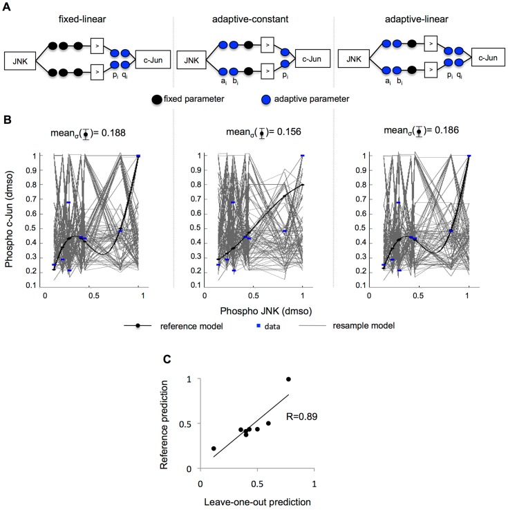
Figure 4. Data-derived sensitivity analysis confirms accuracy and flexibility of approach.

Three formalisms were compared. (A) The schematic left represents the approach presented here, with fixed premise parameters a_i, b_i and number of rules (black circles) and free linear consequent parameters p_i and q_i (blue circles) for each rule i (see equation 2). A zero-order Takagi-Sugeno fuzzy logic system is represented in the center schematic, which features the same input MFs –with free parameters here- and simpler consequent MFs, i.e a constant, with a single free parameter. The right-hand schematic shows the same setup as the left one, with the difference that no parameter was fixed. (B) 100 bootstrapped datasets, i.e. resampled with repetition, were used to train 100 models implemented with each setup (grey curves). The reference model was trained to the full original dataset (black curves for the model, blue dots for the experimental data). The standard deviation σ for the model simulation at each data point was calculated across the 100 bootstrapped models. As a signature of accuracy and flexibility, the mean of the deviation mean_σ for all data points was next calculated. While both the adaptive-linear and fixed-linear show an ability to adapt to the different datasets (mean_σ(fixed-linear) = 0.188 and mean_σ(adaptive-linear) = 0.186), the adaptive-constant setup exhibited a less flexible performance (center, mean_σ(adaptive-constant) = 0.156) confirming that the consequent parameters outweigh the premise parameters in impact. (C) Leave-one-out cross-validation was performed to assess over-fitting by splitting the eight JNK-c-Jun pairs into two sets, leaving a single pair of observations as test set and the remaining time points as training set. A gFIS was fit to the training set and a prediction was made for the excluded observation using its JNK value for all eight data pairs, yielding one prediction for each differently trained model (x axis). Next, a gFIS was trained to the full dataset, creating a reference model that was used to make a prediction for each observed JNK value (y axis). Confirming model predictivity, the predictions of the reference model correlated largely with the test predictions (R = 0.89).