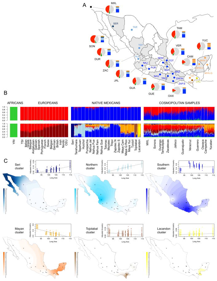
Fig. 2.

Mexican population structure. (A) Map of sampled populations (detailed in Table S1) and admixture average proportions (Table S5). Dots correspond to Native Mexican populations color-coded according to K=9 clusters identified in B (bottom), and shaded areas denote states in which cosmopolitan populations were sampled. Pie charts summarize per-state average proportions of cosmopolitan samples at K=3 (European in red, West African in green, and Native American in gray). Bars show the total Native American ancestry decomposed into average proportions of the native subcomponents identified at K=9. (B) Global ancestry proportions at K=3 (top) and K=9 (bottom) estimated with ADMIXTURE including African, European, Native Mexican, and cosmopolitan Mexican samples (Tables S1–S2). From left to right Mexican populations are displayed North-to-South. (C) Interpolation maps showing the spatial distribution of the six native components identified at K=9. Contour intensities are proportional to ADMIXTURE values observed in Native Mexican samples, with crosses indicating sampling locations. Scatter plots with linear fits show ADMIXTURE values observed in cosmopolitan samples versus a distance metric summarizing latitude and longitude (long axis) for the sampled states. From left to right: Yucatan, Campeche, Oaxaca, Veracruz, Guerrero, Tamaulipas, Guanajuato, Zacatecas, Jalisco, Durango, and Sonora. Values are adjusted relative to the total Native American ancestry of each individual (9).