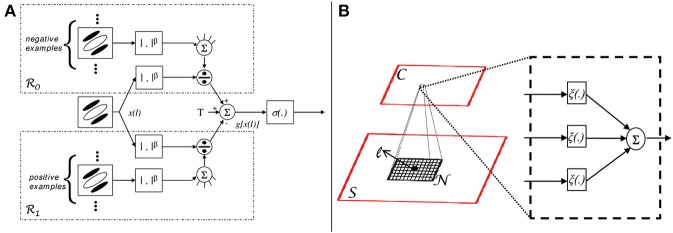
Figure 2.

Discriminant saliency computations. (A) Simple cell (S unit). A unit of receptive field centered at location l computes a feature response x(l). This is then rectified, differentially divisively normalized by feature responses from areas R₀ and R₁, and fed to a sigmoid. The responses from the two areas act as training sets for the binary classification of x(l). More precisely, responses in R₀ (R₁) act as training examples for the negative (positive) class. The output g[x(l)] of the differential divisive normalization operator is the log-likelihood ration for the classification of x(l) with respect to the two classes (under the assumption of GGD statistics), as in (9). The sigmoid finally transforms this ratio into the posterior probability of the positive class, as in (3). (B) Complex cell (C unit). The bottom plane symbolizes the output of a layer of S-units, the top one the output of a layer of C-units. S-unit responses within a neighborhood N(l) are passed through non-linearity ξ(x) and pooled additively, to produce the response of a C unit. This implements the saliency measure of (8).