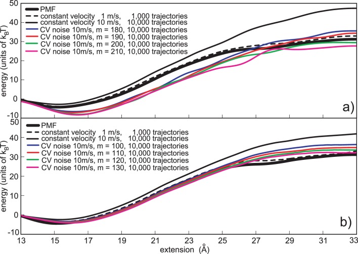
Figure 3. Constant variance noise based reconstructions.
a) Jarzynski PMF estimates based on the constant variance noise protocol. The Gaussian noise was applied with the 10 m/s pulling velocity. Four noise amplitudes are depicted, m = 180, 190, 200 and 210. b) Cumulant expansion PMF estimates based on the constant variance noise protocol. The Chi-square noise was applied with the 10 m/s pulling velocity. Four noise amplitudes are depicted, m = 100, 110, 120 and 130. The estimates based on the normal pulling (1 m/s and 10 m/s) are given for the comparison. In each case depicted the computational cost is the same, i.e., it is analogous to the cost required to generate 10,000 trajectories using normal pulling and 10 m/s velocity.

