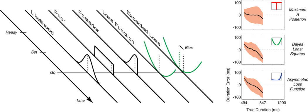
Figure 1.

Left: The participant has to anticipate the “Go” signal after seeing the “Ready” and “Set” preparation signals. Knowing that the variable interval between “Ready” and “Set” is identical to the interval between “Set” and “Go”, what is the best strategy to predict the occurrence of the “Go” signal? A Bayesian decision maker answers this question by combining several pieces of information. The first piece of information is the likelihood function that represents the probability of making the measurement the participant has just made on the present duration from “Ready” to “Set” given various possible true durations The likelihood can be seen as the uncertainty of the measurement. The second piece of information is the prior probability distribution that represents the accumulated knowledge of interval durations over past races run with this race official. The product of the likelihood function and the prior distribution determines the posterior distribution and represents the probability of various possible estimates of the interval duration given the current measurement. The final piece of information is the loss function that represents the costs associated with correct and incorrect estimates. Combining the posterior distribution with the loss function gives the expected loss that represents the anticipated cost associated with different duration estimations. The minimum of the expected loss corresponds to the optimal decision for a Bayesian decision maker, indicated by the dashed green line. This optimal time is negatively biased relative to the veridical duration as a result of the prior (most previous races had a shorter duration). Right: Three Bayesian models of duration estimation for true durations chosen from the lowest range of durations used in the Jazayeri and Shadlen study (ref. 1). Each plot shows the mean ( one standard deviation) estimates over 1000 simulated races. For maximum a posteriori MAP) estimation, the loss function penalizes all errors equally (see top-right inset). This model is accurate (weakly biased) but not very precise (large variability of the estimates). For Bayes least squares (BLS) estimation, the loss function is quadratic. This model has smaller variability but larger bias, especially for long durations. The large bias for long durations is the result of the increased uncertainty of the likelihood function for longer durations (the scalar variability property). The last model is based on an asymmetric loss function that penalizes late starts more than early starts. This model shows similar accuracy and precision to the BLS model. Note in particular the larger biases for longer durations that are now the result of the high cost for overestimates, even if the participant’s internal model of likelihood is incorrect (no scalar variability). Different combinations of likelihood, prior and loss function can lead to similar predictions.