Figure - PMC

Skip to main content

An official website of the United States government

Here's how you know

Here's how you know

Official websites use .gov
A .gov website belongs to an official government organization in the United States.

Secure .gov websites use HTTPS
A lock ( ) or https:// means you've safely connected to the .gov website. Share sensitive information only on official, secure websites.

View full-text article in PMC

. 2014 Sep 24;8:176. doi: 10.3389/fnsys.2014.00176

Search in PMC
Search in PubMed
View in NLM Catalog
Add to search

Copyright © 2014 Botcharova, Farmer and Berthouze.

This is an open-access article distributed under the terms of the Creative Commons Attribution License (CC BY). The use, distribution or reproduction in other forums is permitted, provided the original author(s) or licensor are credited and that the original publication in this journal is cited, in accordance with accepted academic practice. No use, distribution or reproduction is permitted which does not comply with these terms.

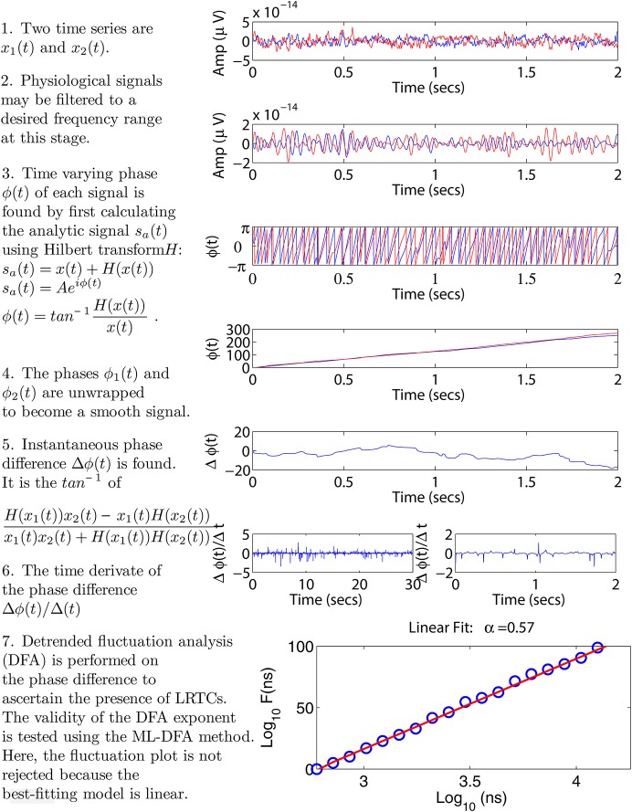
PMC Copyright notice

Step-by-step illustration of the proposed method. We use two sample MEG signals from the left and right motor cortex, displayed throughout panels 1–4 in red and blue, respectively. Panel 2 shows an optional bandpass filtering step. In panel 3 the instantaneous phases of the two time series are calculated using the Hilbert transform. Panel 4 shows the unwrapped phases leading to a time-varying phase difference displayed in panel 5. In panel 6, the rate of change of this phase difference is calculated. This step is illustrated using two plots, each showing a different time scale in the x-axis. These two time scales correspond to the minimum and maximum window sizes used in the DFA analysis, see Section 2.4. Panel 7 shows the resulting DFA fluctuation plot. The validity of this plot is determined using ML-DFA, see Section 2.5. In this case, the validity of the DFA plot was confirmed, with a DFA exponent of 0.57.