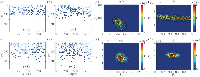
Figure 2.

(a–d) Typical evolution of the discrete simulation described in §3.2, generated with (P_m, P_p) = (0.25, 2 × 10⁻³), presented at time (a) t = 0 h, (b) t = 4 h, (c) t = 8 h and (d) t = 12 h. (e–h) Calculated posterior distribution obtained from a summary statistic generated with (P_m, P_p) = (0.25, 2 × 10⁻³) using (e) the pair correlation function q(i), (f) the number of cells N, (g) the counts of pair distances c(i) and (h) K, the combination of q(i) and N as the summary statistic. The details of the process to obtain the distributions are given in the electronic supplementary material. In brief, is the maximum difference between the summary statistics for θ to be accepted, Γ is the width of the distribution of potential step sizes in the ABC-MCMC algorithm and M is the total number of steps attempted. Parameter values used were (e) , (f) , (g) and (h) . values were chosen such that the posterior distribution did not significantly change if was reduced (electronic supplementary material). For all simulations τ = 1/24 h, Γ = (10⁻¹, 10⁻³), M = 10⁶, N(0) = 100, Y₀ = 10. Red areas indicate high relative frequency while blue areas indicate low relative frequency. All simulation data are insensitive to τ. The white squares represent the parameter values used to generate the synthetic data.