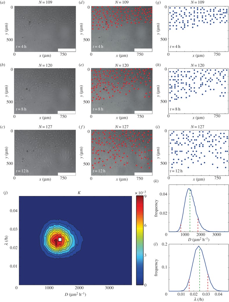
Figure 4.

(a–c) Typical experimental images of a scratch assay at (a) t = 4 h, (b) t = 8 h and (c) t = 12 h. (d–f) Experimental images of a scratch assay with the position of cells indicated (red squares) at (d) t = 4 h, (e) t = 8 h and (f) t = 12 h. (g–i) The position of cells when mapped onto a lattice at (g) t = 4 h, (h) t = 8 h, (i) t = 12 h. (j) Posterior distribution calculated using K, which is the average of q(i) and N, as a summary statistic and . The details of the process to obtain the distribution are given in the electronic supplementary material. In brief, is the maximum difference between the summary statistics for θ to be accepted, Γ is the width of the distribution of potential step sizes in the ABC-MCMC algorithm and M is the total number of steps attempted. For all simulations, τ = 1/24 h, Γ = (10⁻¹, 10⁻³), M = 10⁶, N(0) = 102, Y₀ = 10. Red areas indicate high relative frequency while blue areas indicate low relative frequency. was chosen such that the posterior distribution did not significantly change if was reduced (electronic supplementary material). The white square represents the mean parameter values, (D, λ) ≈ (1350 μm² h⁻¹, 2.5 × 10⁻² h⁻¹). All simulation data are insensitive to τ. (k) Posterior distribution of λ obtained by averaging over D with the mean, λ = 2.5 × 10⁻² h⁻¹, (dashed green) and 90% credible interval, (1.7 × 10⁻²−3.1 × 10⁻²)/h (dashed red) superimposed. (l) Posterior distribution of D obtained by averaging over λ with the mean, D = 1350 μm² h⁻¹, (dashed green) and 90% credible interval, (675−1800) μm² h⁻¹ (dashed red), superimposed.