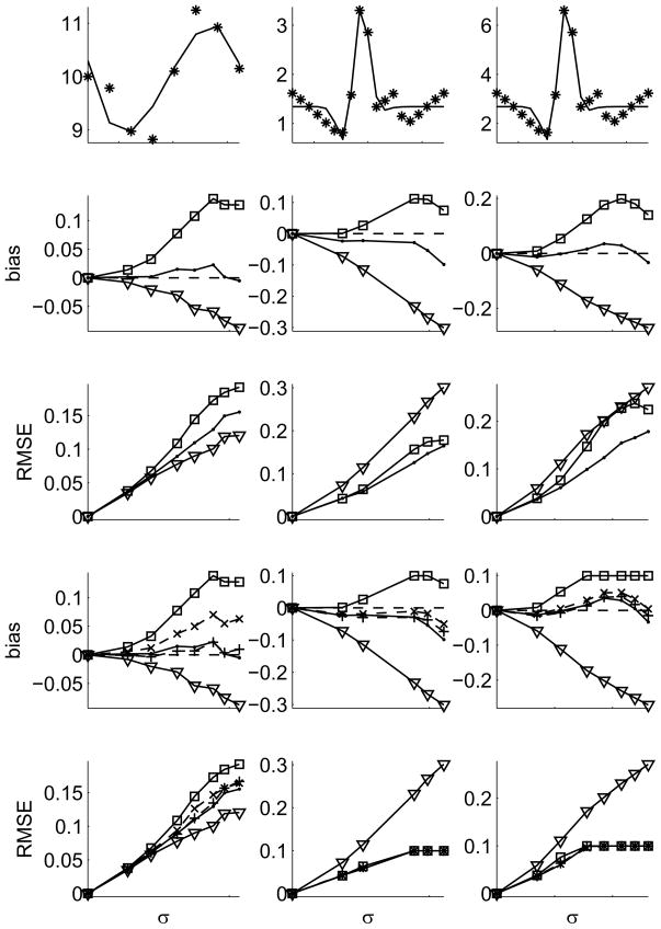
Figure 1.
Simulation results: Left column: a 3rd degree polynomial is fit to noise data drawn from an underlying sine-function. Center & Right column: a Gabor function is fit to noisy data around a linear combination of three Gaussians – two ‘excitatory’ and one ‘inhibitory’. Left & Center: Gaussian noise, Right: Gamma distributed noise (Fano factor of 2). First row: data (stars) and model (lines) are shown in the noise-free condition. Their true VE is 77% and 90%, respectively. Rows 2–5: bias (defined as estimated minus true VE) and RMSE are shown as a function of noise σ. The traditional estimator is shown by triangles, the Sahani-Linden correction by squares, our estimator from eq. (8) by dots. Rows 4 & 5: VE measures were restricted to the range 0 to 1. Estimators with conditioning (eq. 9) optimized for bias (+) and MSE (x), both dashed. Restricting VE to 0 ≤ ν ≤ 1 is the reason for the plateau in the bias of the Sahani-Linden estimator. In all panels data samples with insignificant variation in the data (pANOVA > 0.05) were excluded from the analysis. Note the different scales in each panel.

