Abstract
Background
Amnestic mild cognitive impairment (aMCI) is considered to be a transitional stage between healthy aging and Alzheimer's disease (AD), and consists of two subtypes: single-domain aMCI (sd-aMCI) and multi-domain aMCI (md-aMCI). Individuals with md-aMCI are found to exhibit higher risk of conversion to AD. Accurate discrimination among aMCI subtypes (sd- or md-aMCI) and controls could assist in predicting future decline.
Methods
We apply our novel thickness network (ThickNet) features to discriminate md-aMCI from healthy controls (NC). ThickNet features are extracted from the properties of a graph constructed from inter-regional co-variation of cortical thickness. We fuse these ThickNet features using multiple kernel learning to form a composite classifier. We apply the proposed ThickNet classifier to discriminate between md-aMCI and NC, sd-aMCI and NC and; and also between sd-aMCI and md-aMCI, using baseline T1 MR scans from the Sydney Memory and Ageing Study.
Results
ThickNet classifier achieved an area under curve (AUC) of 0.74, with 70% sensitivity and 69% specificity in discriminating md-aMCI from healthy controls. The same classifier resulted in AUC = 0.67 and 0.67 for sd-aMCI/NC and sd-aMCI/md-aMCI classification experiments respectively.
Conclusions
The proposed ThickNet classifier demonstrated potential for discriminating md-aMCI from controls, and in discriminating sd-aMCI from md-aMCI, using cortical features from baseline MRI scan alone. Use of the proposed novel ThickNet features demonstrates significant improvements over previous experiments using cortical thickness alone. This result may offer the possibility of early detection of Alzheimer's disease via improved discrimination of aMCI subtypes.
Keywords: Mild cognitive impairment, Cortical thickness, Network, ThickNet, Early detection, Alzheimer
Highlights
-
•
First structural covariance study on amnestic MCI subtypes and controls
-
•
Utilizes fusion of novel ThickNet features from baseline MRI scans alone
-
•
Proposed method improves discrimination power between md-aMCI & controls.
-
•
Suggests ThickNet features can capture subtle changes in early stages of MCI
-
•
Quantitative comparison of classification performance among subtypes of aMCI and controls
1. Introduction
Recent reports suggest that the amyloid pathology may begin up to 20 years before any clinical symptoms appear (Amieva et al., 2008; Braak and Braak, 1991; Braak and Del Tredici, 2011). This highlights the importance of preclinical detection, which still stands as a challenge (Cuingnet et al., 2011). Therefore, there is an urgent need for the development of reliable computer-assisted tools for predicting the conversion in mild cognitive impairment (MCI) due to AD.
The progression rates of clinically-diagnosed mild cognitive impairment (MCI) to dementia are reported to be about 12% per annum (Petersen, 2009). Amnestic subtype of MCI (aMCI) is found to have the highest conversion rate to AD as compared to other dementias (Yaffe et al., 2006). Researchers have categorized aMCI into two broad sub-types of aMCI, based on the number of domains impaired: single-domain (sd-aMCI) and multiple-domain (md-aMCI) subtypes. There is evidence to suggest that md-aMCI is the most likely subtype to progress to AD (Bäckman et al., 2004) and to dementia (Alexopoulos et al., 2006; Brodaty et al., 2013). Moreover, an association between prior subtype of MCI and subsequent progression to a particular dementia is also reported (Yaffe et al., 2006). Hence differential identification of aMCI subtypes, and their relation to specific dementia diagnoses and differential rates of conversion to dementia is worth investigating (Yaffe et al., 2006).
Structural MRI (sMRI) is a widely available noninvasive method that can capture atrophy in the brain structures in terms of subcortical volumetry/shape (Beg et al., 2013; Cuingnet et al., 2011; P. Raamana et al., 2014; Raamana et al., 2014a) as well as cortical thickness features (Cuingnet et al., 2011; Eskildsen et al., 2013; Julkunen et al., 2010; Raamana et al., 2014b). Hence it would be of prognostic value to develop imaging biomarkers, based on baseline structural MRI alone, which can accurately discriminate between the multiple-domain subtype of aMCI and controls.
Previous work thus far mainly focused on analyzing the group differences i.e. regional differences in gray matter loss or cortical thinning. Initial attempts to study the group differences among normal controls (NC), sd-aMCI and md-aMCI were based on voxel-based morphometry (Bell-McGinty et al., 2005; Brambati et al., 2009; Whitwell et al., 2007), with few studies analyzing cortical thickness (Fennema-Notestine et al., 2009; Seo et al., 2007). When comparing sd-aMCI or md-aMCI relative to controls, most of the studies reported differences in medial temporal and inferior temporal lobes (Brambati et al., 2009; Whitwell et al., 2007), which is expected. In the same experiments, Seo et al. (2007) and Fennema-Notestine et al. (2009) reported differences in precuneus as well, suggesting the importance of precuneus as a way to detect early stage atrophy caused by AD. When comparing sd-aMCI relative to md-aMCI, Bell-McGinty et al. (2005) reported a significant loss of volume of the left entorhinal cortex and inferior parietal lobe, whereas Seo et al. (2007) reported cortical thinning in the left precuneus. In summary, these studies suggest that moderate differences exist among the subtypes, and that the structural alterations precede the development of AD (Bell-McGinty et al., 2005). They also suggest that sd-aMCI and md-aMCI clinical subtypes could possibly represent increasing severity points along the continuum between normal aging and AD (Bäckman et al., 2004; Brambati et al., 2009).
The reports from previous studies were on the existence of group-differences among the aMCI subtypes, and where the differences exist, they improve our understanding of the early stage changes caused by AD. However, the sample sizes examined have been small (except for Fennema-Notestine et al., 2009; Whitwell et al., 2007) and unbalanced e.g. 9 sd-aMCI, 22 md-aMCI, and 61 NC in Seo et al. (2007), 9 sd-aMCI, 28 md-aMCI and 47 NC in Bell-McGinty et al. (2005) and 88 sd-aMCI, 25 md-aMCI, and 145 NC in Whitwell et al. (2007). A balanced sample i.e. equal representation for each class in the cohort, is important to ensure that the primary class of interest is not severely underrepresented (Wallace et al., 2011). In a study where the goal is to identify which patients are at increased risk of conversion to dementia, it is important that aMCI (both single and multiple domain subtypes) group is not underrepresented, as in the case of Bell-McGinty et al. (2005), Seo et al. (2007), and Whitwell et al. (2007). Furthermore, it is important to evaluate the diagnostic utility of these measures, which none of the aforementioned studies have assessed based on MRI measures (Bell-McGinty et al., 2005; Brambati et al., 2009; Fennema-Notestine et al., 2009; Seo et al., 2007; Whitwell et al., 2007).
In this study, we propose a novel ThickNet-based classifier for detection of md-aMCI. Our ThickNet fusion method has been previously tested on ADNI dataset for the detection of prodromal AD (P. Raamana et al., 2014). This method utilizes imaging biomarkers based on differential changes in cortical thickness, taking into account pair-wise differences between cortical surface patches. As there is tremendous variability of cortical thickness across the population, the signature of the disease is much more visible in cortical thickness gradients taken between different brain regions, for example anterior–posterior gradients in AD as AD is known to affect cortices such as the medial temporal lobes, the precuneus, parietal areas, entorhinal cortex preferentially and early in the course of the disease. In order to capture such inter-regional gradients (or rather co-variation in general), we formulated these network features. These features will likely complement existing features for early detection based on cortical thickness. These thickness network (ThickNet) features are combined using probabilistic multiple kernel learning approach to form a composite ThickNet classifier. This classifier significantly improves the predictive power in discriminating md-aMCI from NC, compared to the mean thickness values alone (Raamana et al., 2014b). We also show that our method improves the predictive power in the sd-aMCI vs. NC and sd- vs. md-aMCI classification experiments.
2. Materials and methods
2.1. Participants
The study sample was part of the Sydney Memory and Ageing Study (MAS) program, which comprises community-dwelling, non-demented individuals recruited randomly through electoral roll from two electorates of East Sydney, Australia. Please refer to Brodaty et al. (2013) and Sachdev et al. (2010) for complete details about this study. To be eligible, participants needed to be aged between 70 and 90 years old, sufficiently fluent in English to complete the psychometric assessment and were able to consent to participate. Participants were excluded if they had a previous diagnosis of dementia, psychotic symptoms or a diagnosis of schizophrenia or bipolar disorder, multiple sclerosis, motor neuron disease, developmental disability, progressive malignancy (active cancer or receiving treatment for cancer, other than prostate non-metastasized, and skin cancer), or if they had medical or psychological conditions that may have prevented them from completing assessments. Participants were excluded if they had a Mini-Mental Statement Examination (MMSE; Anderson et al. (2007), Folstein et al. (1975)) score of less than 24 adjusted for age, education and non-English speaking background at study entry, or if they received a diagnosis of dementia after comprehensive assessment. The study was approved by the Ethics Committee of the University of New South Wales. The demographics for the current study sample are listed in Table 1.
Table 1.
Demographics of aMCI and normal subjects included in this study.
| Diagnostic group | Total N | Age in years Mean (SD) |
Gender | Education in N years Mean (SD) |
|---|---|---|---|---|
| NC | 42 | 78.57 (4.13) | 17 M + 25 F | 11.97 (3.10) |
| sd-aMCI | 38 | 79.92 (4.87) | 25 M + 13 F | 12.68 (3.53) |
| md-aMCI | 32 | 78.63 (4.44) | 17 M + 15 F | 11.52 (3.84) |
2.2. MAS subsample and cognitive assessments
Participants received a comprehensive neuropsychological assessment examining the cognitive domains of memory, language, attention/processing speed, visuo-spatial function and executive functions (see Table 2 for listing of test measures). Participants were classified as having MCI according to the latest international consensus diagnostic criteria and if all of the following criteria were met — a cognitive complaint from the participant or a knowledgeable informant, cognitive impairment on objective testing, absence of dementia, and normal function or minimal impairment in instrumental activities of daily living. Cognitive impairment was defined as a test performance of 1.5 standard deviations (SDs) or more below published normative values (demographically adjusted where possible — Table 2). Participants were considered impaired in a domain if at least one measure in the domain was impaired. In this study, only amnestic type of MCI is included. If the impairment was restricted to the memory domain, it was classified as single-domain amnestic MCI (sd-aMCI). If an additional cognitive domain was impaired, it was classified as multiple-domain amnestic MCI (md-aMCI). Participants from non-English speaking background were excluded from the MCI groups because of the questionable validity of applying standard normative data to establish cognitive impairment in non-native English speakers (Kochan et al., 2010). We additionally excluded subjects whose cortical parcellation did not meet our quality control. Within the quality controlled subset, we randomly selected a subset of controls that matched in age and size with aMCI. The final selection consisted of 38 sd-aMCI, 32 md-aMCI and 42 age-matched NC.
Table 2.
Neuropsychological tests used for MCI classifications.
| Cognitive domain | Test | Normative data source and demographic adjustments |
|---|---|---|
| Premorbid intelligence | National adult reading test (NART) | No adjustments |
| Attention/processing speed | Digit symbol-coding | Age |
| Trail making test A | Age and education | |
| Memory | Logical memory story A delayed recall | Education |
| RAVLT | Age | |
| RAVLT total learning, trials 1 to 5 | ||
| RAVLT short-term delayed recall; trial 6 | ||
| RAVLT long-term delayed recall; trial 7 | ||
| Benton visual retention test recognition | Age and education | |
| Language | Boston naming test Ñ 30 items | Age |
| Semantic fluency (animals) | Age and education | |
| Visuospatial | Block design | Age |
| Executive function | Controlled oral word association test (FAS) | Age and education |
| Trail making test B | Age and education |
Please refer to Sachdev et al. (2010) for complete details on normative data sources and related references.
2.3. Image acquisition
The participants were scanned using a 3 T Intera Quasar scanner initially, followed by a 3 T Achieva Quasar Dual scanner, both manufactured by Philips Medical Systems, Best, The Netherlands. There was no alteration in acquisition parameters for T1-weighted sequences for both the scanners: TR = 6.39 ms, TE = 2.9 ms, flip angle = 8°, matrix size = 256 × 256, FOV = 256 × 256 × 190, and slice thickness = 1 mm with no gap between; yielding 1 × 1 × 1 mm3 isotropic voxels.
The use of different scanners was due to reasons beyond investigator's control and any systematic bias arising from the scanner change is unlikely given that participant recruitment was random. There were no significant differences found between the two scanners in cortical features extracted from five healthy subjects in the Sydney MAS cohort scanned on both scanners (Liu et al., 2010). Even though there were some cohort differences across the two scanners (at age scan: scanner 1 = 77.9, scanner 2 = 79.0, p = 0.003; years of education: scanner 1 = 11.4, scanner 2 = 12.2, p = 0.013; male/female ratio: scanner 1 = 125/160, scanner 2 = 120/137, p = ns; the final selection of subjects in Section 2.2 is part of this larger cohort), previous studies have suggested that when vendor, field strength, and acquisition parameters remained unchanged, data collected during scanner upgrades could be pooled (Stonnington et al., 2008). Moreover, in the subset being studied, the number of subjects in each diagnostic group belonging to the two scanners is evenly distributed across the two scanners (see Table 3), indicating that the chances of biases are reduced.
Table 3.
Number of subjects per scanner per diagnostic class.
| Class | S1 | S2 |
|---|---|---|
| NC | 20 | 22 |
| sd-aMCI | 18 | 20 |
| md-aMCI | 15 | 17 |
2.4. Thickness measurement and processing
Initial cortical reconstruction and volumetric segmentation of the whole brain were performed with the Freesurfer image analysis suite (Dale et al., 1999; Fischl et al., 1999) to obtain pial and WM/GM surfaces. The resulting cortical parcellations were quality controlled whenever possible — see Appendix A for more details. In the space between these surfaces, a discrete approximation of Laplace's equation was solved (Gibson et al., 2009; Yezzi, 2003) using the tools developed by our group. Streamlines of this harmonic function define corresponding points on the surfaces, and the Euclidean distance between these points defines the cortical thickness. In order to perform group-wise-analysis, we registered the surface of each subject in the study to the surface of a common atlas (derived from averaging over 80 healthy subjects) using the tools from Fischl et al. (2004). This atlas was not involved in the thickness measurement step, but was only used for group-wise registration. Registration to a common atlas establishes vertex-wise correspondence and enables group-wise analysis of the differences in thickness. Finally, cortical thickness was smoothed with a 10-mm full width at half height Gaussian kernel to improve the signal-to-noise ratio and statistical power for subsequent analysis (Lerch and Evans, 2005).
2.5. Novel dimensionality reduction
Each cortex surface contained 327,684 vertices in the whole brain and we have a limited number of subjects. To avoid the curse of dimensionality, we partitioned each cortical label (such as posterior cingulate etc. from the 68 Freesurfer-derived cortical labels) containing thousands of vertices into a small number (say 10) of partitions by clustering vertices, within each label, using k-means clustering of vertex coordinates. The thickness feature for each sub-partition is defined as the average thickness across vertices in that partition. This novel approach not only reduces the dimensionality of the features but also does it in anatomically meaningful way, as opposed to other dimensionality reduction methods (such as PCA) which transform the features to an entirely different space which may lack physical meaning and anatomical relevance. Note that clustering is done within each Freesurfer label, which prohibits linking vertices across different labels. Moreover, the vertex density of Freesurfer parcellation is sufficiently even and high to satisfy the k-means assumptions (Lee et al., 2006), and visual verification of partitioning confirmed the desired outcome. Visualization of such a subdivision of the cortex into 680 partitions is shown in Fig. 1. As they are all registered to a common atlas, this subdivision of the cortex is propagated into the cortical surface of each subject to establish correspondence for our analysis.
Fig. 1.
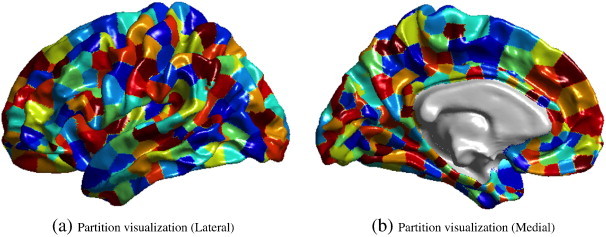
Visualization of the partitions on the atlas surface in the medial view (a) and lateral view (b), when TNP = 680.
It is worth noting that certain trade-offs exist in deciding the total number of partitions (TNP) for this method. When we choose to average across the entire Freesurfer label (which can be quite large covering many gyri and sulci), we may lose the discriminatory signal. In contrary, when the TNP is excessively large e.g. over 5000, we risk the curse of dimensionality as well as making the method overly sensitive to noise. Hence we study the performance of this method for different values of TNP = 340, 680, 1020, 1360 and 1700, to avoid making an arbitrary choice.
2.6. Thickness network (ThickNet) features
Once the pial surface is partitioned into large number of small sub-partitions (thought of as nodes), a network (graph) is constructed by establishing a link between two nodes if the absolute difference in mean thicknesses is below a specified threshold. The term network is used here in the abstract sense to mean a mathematical graph and not a functional/structural network connected by physical fiber tracts or connections. From this binary undirected graph, we compute thickness network measures – we term them ThickNet features – such as nodal degree, betweenness centrality and clustering coefficient to represent each individual brain. ThickNet measures are intrinsic to each subject and offer insight into regional correlations in cortical thinning. The extraction of ThickNet features is illustrated in the form of a flowchart in Fig. 2, which is described in detail in the rest of this section.
Fig. 2.
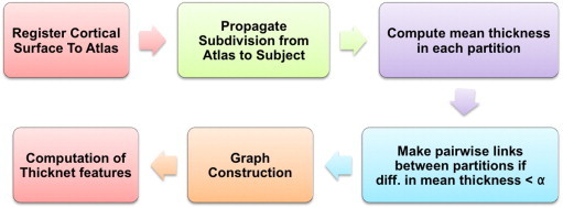
Flow chart describing the steps involved in the extraction of ThickNet features. Once the pial surfaces from all the subjects are registered to a common atlas, we subdivide the cortex of the atlas surface into a fixed number of partitions (or patches). This subdivision is propagated into cortical surface of each subject and mean thickness within each partition is computed for all the patches in every subject. Based on the similarity in thickness, links are defined between various pairs of partitions with difference in mean thickness below a certain threshold. The Boolean link status between all the pairwise connections forms the adjacency matrix of the graph. From this graph, we compute various ThickNet features. Please refer to Section 2.6 for a detailed description.
Suppose N is the set of all nodes in the network (the number of nodes n = 68·NPP, NPP = number of partitions per Freesurfer label in each of the 68 Freesurfer labels) and L is the set of all links in the network (l = number of links). Note N equals TNP, which is the total number of partitions in each subject's cortical surface. Let (i,j) be a link between nodes i and j (i, j ∈ N) and aij is the link status between i and j: aij = 1 when link (i,j) exists; aij = 0 otherwise. A link is defined between i and j, if |MTi − MTj| < = α, where MTx represents the mean thickness in the node x, x ∈ N. Here α is the threshold to establish a link. A lenient threshold (α > 0.5 mm) allows large number of links in the cortex, whereas a stringent threshold (α ≤ 0.5 mm) allows relatively few links. It is important to note that spatial (or topographic) distance or adjacency is not part of the linking criteria, as the method searches all possible pairwise links between all cortical sub-partitions.
We chose to utilize nodal degree (measure of how connected each node is), betweenness centrality (measure of centrality) and clustering coefficient (measure of segregation) from the binary graph as properties to describe the network (Rubinov and Sporns, 2010). In brief, for a given node i, these are defined as
| (1) |
| (2) |
| (3) |
where is the number of triangles around node i; ρhj is the number of shortest paths between h and j and ρhj(i) is the number of shortest paths between h and j that pass through i. Please note that ki in Eq. (3) is the nodal degree defined in Eq. (1).
Intuitively, the degree of an individual node is equal to the number of links connected to that node, which therefore reflects the level of interaction of that node in the network. It is hypothesized that there are central nodes which participate in many short paths in the brain network. Betweenness centrality measures the fraction of all shortest paths in the network that pass through a given node. It is also known that human brain segregates specialized processing into interconnected groups of brain regions (clusters) — clustering coefficient measures the clustering connectivity around a given node.
The ThickNet features for the NC and md-aMCI classes, in the form of group-differences i.e. mean(NC)–mean(md-aMCI) at each partition, are visualized in Fig. 3.
Fig. 3.
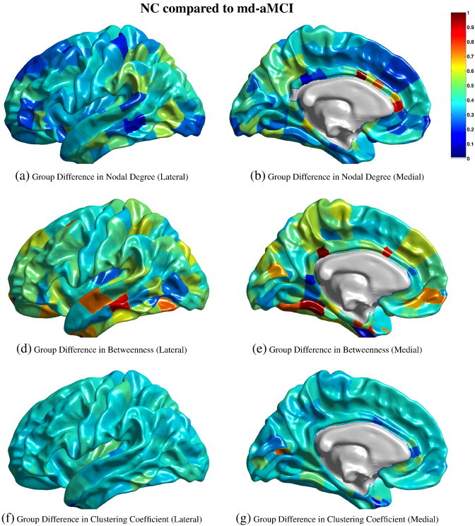
Visualization of the differences in group means, i.e. mean(NC)–mean(md-aMCI) at each partition, of the ThickNet features when TNP = 340 and α = 0.20. The left column presents the medial view and the right column presents the lateral view, of the group differences in each feature. The values of each feature in (a) to (g) are normalized to [0,1] to enable comparison across features. These values do not have any applicable units. Note that these visualizations are obtained from a fixed partial view of the cortex, and presented here for illustration purposes only, and may not be indicative of their predictive performance.
3. Evaluation of predictive utility
The ThickNet features reveal different properties of the regional links in thickness in the human brain. In order to maximize their utility for the early detection of AD, these features can be fused to form a composite set of features. Multiple kernel learning (MKL) is a natural choice for such a fusion of different features for the classification task. The procedure to evaluate the predictive utility is described in the following sections, and also summarized using a flowchart in Fig. 4.
Fig. 4.
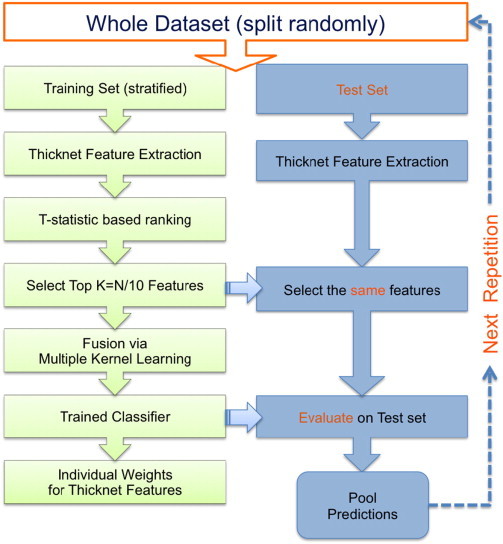
Flowchart illustrating the performance evaluation procedure utilized in this study. The training set is stratified in the sense that there is no class-imbalance (all the classes are equal in size), to limit any bias towards one particular class. Please note that this procedure is repeated 100 times. In each repetition, the performance metrics are computed based on the predictions from the corresponding test set only. In other words, we do not pool predictions across different repetitions — which may invalidate the computation of AUC. That would be invalid because the prediction scores in different repetitions are obtained from different classifiers, which may not be comparable or calibrated.
3.1. Probabilistic multiple kernel learning
One such method is the variational Bayes probabilistic MKL (VBpMKL) which has been successfully applied to protein fold recognition (Damoulas and Girolami, 2008). This method combines multiple feature spaces, allowing a different kernel (e.g. gaussian, polynomial) for each feature space to embed them in a high-dimensional similarity space, using a variational Bayes approximation to form a composite kernel. This composite kernel is fed to a multi-class model which applies Bayes theorem to learn the significance of each feature, as well as the kernel weights and kernel parameters automatically, without resorting to ad hoc parameter tuning. VBpMKL outputs probability estimates of membership to each class for each test subject, from which we can compute performance metrics (such as accuracy) as well as construct receiver operating characteristic (ROC).
3.2. Feature selection
Prior to fusion, further feature selection is done (within each feature set separately), by ranking each partition by its two-sample t-statistic computed from the training set alone. All the partitions are ranked by their t-statistic and the top K partitions are selected for training the classifier. We computed t-statistic with the alternative hypothesis that means are not equal assuming the variances are not equal, using the following formulae:
| (4) |
Here s2 is an unbiased estimator of the variance of the two samples X1 and X2. and ni are the mean and the number of participants in each sample i = 1,2 respectively.
3.3. Largest reduced dimensionality to avoid over fitting
We propose a novel approach derived from analytical results to set the largest dimensionality. There is an empirical relationship between the number of features (K) used to train the classifier and the minimum size of the training sample needed to avoid the curse of dimensionality, which is that for K number of features and small probability of error p(e), the minimum sample size required (Fitzpatrick and Sonka, 2000). If one would like to keep p(e) below 5% with K features, we need at least Nmin = K/(2 ∗ 0.05) = K ∗ 10 subjects for training. We use this relation to determine the maximum number of features that can be used to train the classifier with an Ntrain number of samples in the training set i.e. Kmax = Ntrain/10. This would give a Kmax = 8, 7 and 7 for the three pairs NC vs. sd-aMCI, NC vs. md-aMCI and sd-aMCI vs. md-aMCI respectively, when using the evaluation method to be described below in Section 3.4. We propose to use this novel approach to set the largest dimensionality to avoid the possibility of over-fitting.
3.4. Repeated Hold-out, Stratified Training set (RHsT)
Using this combination i.e. t-stat feature selection followed by VBpMKL as the classification system, we evaluate its predictive utility using a novel form of repeated holdout method to handle class-imbalance. We eliminate class-imbalance in the training set by first selecting a fixed percentage of subjects from the smallest class, and then selecting the same number from all the classes in the dataset. We denote it as the Repeated Hold-out, Stratified Training set (RHsT) evaluation method. It is stratified in the sense that each class has an equal number of subjects in the training set to eliminate any class imbalance that may arise for typical uses of popular cross-validation methods. In each repetition, we hold out Ntrain subjects from each class for training and reserve the rest for testing the classifier. Here Ntrain is determined by 95% of the smallest class in the experiment. For example, in an experiment with 42 NC subjects and 32 md-aMCI subjects, training set would consist of Ntrain = ⌊0.95 ∗ 32⌋ = 30 samples from NC and md-aMCI. And the testing set would have 12 NC and 2 md-aMCI subjects. In each repetition, we compute the accuracy, sensitivity and specificity as well as area under curve (AUC) by constructing an ROC, from the predictions generated for the corresponding unseen test set. This method is repeated 100 times, each time creating random training/test sets, in order to avoid the bias that can arise from a single training/test sets as in Cuingnet et al. (2011). The mean performance metrics, and their standard deviations, from the 100 repetitions are reported.
3.5. Significance testing of performance improvement
To demonstrate the added value of the proposed ThickNet features, relative to mean thickness (MT) features alone, we performed additional experiments testing the statistical significance of the improvement in classification performance. The classification power of mean thickness features alone, in place of the ThickNet features, is evaluated while keeping the rest of the evaluation procedure (RHsT) the same. We perform significance testing of improvement in AUC using ROC comparison methods described in Witten and Frank (2005). RHsT provides us with 100 estimates of AUC for each repetition of a cross-validation experiment. We utilize these AUC samples for ThickNet and MT features and estimate whether one is significantly better than the other, using a non-parametric Wilcoxon rank-sum test (Hollander et al., 2013).
3.6. Validation on an independent dataset
In this study, we have employed sophisticated cross-validation techniques (see Section 3) and ROC analysis, in order to obtain unbiased and robust estimates of the predictive power of the ThickNet fusion method. Cross-validation (CV) techniques, such as RHsT, is typically employed when there is no separate test set, and CV methods provide us with the closest estimate of the true generalization performance. However we recognize the importance of validation and external replication (Fletcher and Grafton, 2013). Hence, when possible, it is desirable to estimate the performance of the novel method on an independent dataset. Unfortunately, to the best of our knowledge, an independent dataset with compatible diagnostic classes of single and multiple-domain subtypes of amnestic MCI does not yet exist.
We therefore performed the validation experiments on half of the current cohort. We have randomly split the current cohort into two parts: training set (50%) used for optimizing the ThickNet method and validation set (50%) which is entirely kept aside for final evaluation of results. The ThickNet method is optimized using cross-validation based entirely on the training set only (using the same procedure as described in Section 3) to arrive at an optimal configuration (TNP, α) for the ThickNet method. In this way, the optimal model is trained on random half of the study population, and its classification performance is evaluated on the other half. The AUC on the validation set is compared to the results based on the entire cohort in all the three experiments which are presented in Table 6.
Table 6.
Comparison of classification performance of the optimal model on the validation set (50% split), compared to that derived from the entire cohort (unsplit).
| Experiment | Best (TNP, α) |
AUC |
|||
|---|---|---|---|---|---|
| Full cohort | Split cohort | Full cohort | Training set (50%) | Validation set | |
| NC vs. sd-aMCI | 1020, 0.20 | 1360, 0.60 | 0.61 | 0.62 | 0.53 |
| NC vs. md-aMCI | 340, 0.20 | 340, 0.20 | 0.74 | 0.66 | 0.65 |
| sd- vs. md-aMCI | 1360, 0.20 | 1020, 0.20 | 0.67 | 0.69 | 0.62 |
4. Results
The evaluation method as described in Section 3, and graphically summarized in Fig. 4, is applied to the fusion of the following four feature sets: mean thickness (MT), nodal degree (ND), betweenness centrality (BE) and clustering coefficient (CL) at each partition. From our previous experiments on MCI/NC classification (Raamana et al., 2013), we observed the best performance from VBpMKL using a polynomial kernel (3rd degree) for each feature set and thereby fixing it as the kernel of choice for this study. The performance of the fusion method is evaluated in discriminating between md-aMCI and NC. For the sake of comparison, the performance of ThickNet classifier is also evaluated in discriminating between sd-aMCI and NC, as well as between sd-aMCI and md-aMCI.
For each experiment, there are two parameters that change the feature extraction process (of the mean thickness and the three network features): TNP and the link threshold α. Choice of different TNPs can be thought of as selecting a different parcellation scheme (coarse to finer resolution), and selecting different values for threshold α can be thought of as selecting different types of features i.e. weak connections (higher-order features) with lenient α (large tolerance for similarity), and strong connections (lower-order) with stringent α (relatively low tolerance for similarity). To avoid making an arbitrary choice for these parameter values, we have studied the performance of our method for different combinations of TNP and α, with TNP = 340, 680, 1020 and 1360, and α was varied from 0.1 mm to 1.5 mm, in steps of 0.1 mm. The AUCs for all the combinations are visualized in Fig. 5.
Fig. 5.
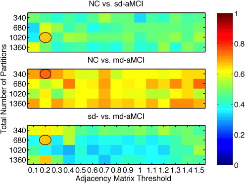
Comparison of AUC obtained from RHsT method for each combination of NPP and α. The combination with the best performance (highest AUC) in each experiment is highlighted with a black oval.
The best performance (highest AUC) of the ThickNet fusion method for different experiments is summarized in Table 4, with different performance metrics and the optimal ThickNet parameters TNP and α. Corresponding ROCs are visualized in Fig. 6, which are constructed by averaging the 100 ROCs obtained from the 100 repetitions of the RHsT, using the vertical averaging method as described in Fawcett (2006).
Table 4.
Best performance (highest AUC) of the ThickNet fusion method for each experiment, in various classification metrics (with their std. deviation from the 100 repetitions of RHsT) describing the performance. The optimal TNP and threshold (α) are noted for each experiment. The optimal values for TNP and α are different because we exhaustively analyzed the performance of the method for various parameter choices in order to find the best model, to avoid making an arbitrary choice.
| Experiment | AUC (SD) | ACC (SD) | SENS (SD) | SPEC (SD) | TNP | α |
|---|---|---|---|---|---|---|
| NC vs sd-aMCI | 0.61 (0.28) | 0.56 (0.22) | 0.75 (0.44) | 0.52 (0.24) | 1020 | 0.20 |
| NC vs md-aMCI | 0.74 (0.27) | 0.62 (0.13) | 0.71 (0.46) | 0.61 (0.14) | 340 | 0.20 |
| sd- vs md-aMCI | 0.67 (0.31) | 0.58 (0.17) | 0.64 (0.48) | 0.57 (0.19) | 1360 | 0.20 |
Fig. 6.
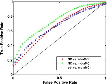
Comparison of ROC curves corresponding to the best performance of ThickNet fusion method in each experiment.
4.1. AUC for different TNP and α
The sensitivity and specificity estimates of the ThickNet fusion classifier, similar to the AUC estimates as visualized in Fig. 5, for different values of TNP and α are presented in Figs. 7 and 8 respectively. These figures show that the performance of our method, in qualitative terms, is robust (insensitive to parameter choices) to different values of the parameters TNP and α. Moreover we notice that these metrics follow the same trends as AUC, when the performance of ThickNet fusion method is compared across the different experiments.
Fig. 7.
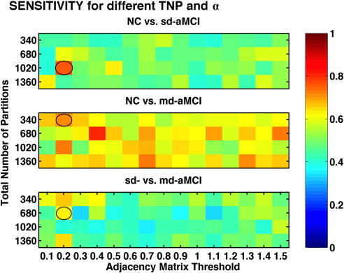
Comparison of sensitivity, for different values of TNP and α, obtained from RHsT method. The combination with the best performance (highest AUC) in each experiment is highlighted with a black oval.
Fig. 8.
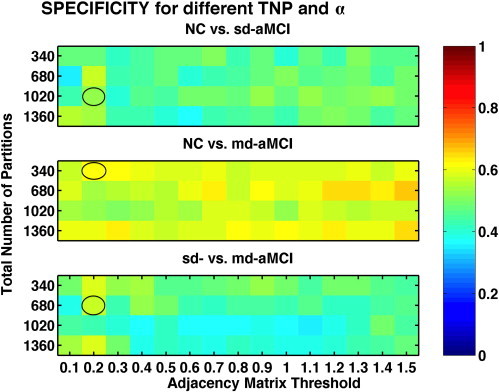
Comparison of specificity, for different values of TNP and α, obtained from RHsT method. The combination with the best performance (highest AUC) in each experiment is highlighted with a black oval.
4.1.1. Individual significance of ThickNet features
For each run of RHsT, we obtain not only the prediction of the test set subjects, but also the significance of each feature set in the fused classifier, estimated by VBpMKL. This allows to gain further insight into the contribution of different feature sets. The average weights from the 100 repetitions of RHsT for the ThickNet features are visualized in Fig. 9, for the three classification experiments.
Fig. 9.
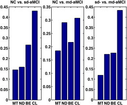
Individual contribution of ThickNet features towards classification in the pMKL framework. Here MT denotes mean thickness, ND denotes nodal degree, BE denotes betweenness centrality and CL denotes clustering coefficient. These results show that all the ThickNet features contributed to discrimination much more than MT, although in varying proportions. CL exhibited the largest weight in all the experiments, demonstrating its significance. Note that the contribution of ThickNet features increased with increasing difficulty of the problem, such as NC vs. sd-aMCI and sd-aMCI vs. md-aMCI, which further asserts their utility for the prognostic applications.
The results of significance testing as described in Section 3.5, of whether the classification improvement offered by ThickNet over mean thickness is significant or not, are shown in Fig. 10 and Table 5. The corresponding ROCs for ThickNet and MT are compared in Fig. 6. Table 5 shows that ThickNet outperformed MT in terms of AUC for all the experiments except CN vs. sd-aMCI.
Fig. 10.
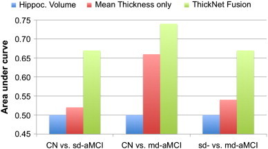
Comparison of performance of the proposed ThickNet fusion method with respect to the baselines such as using mean thickness (MT) only and using hippocampal volume (HV) only. It is immediately obvious that our ThickNet fusion method significantly improved the predictive power (AUC) in detection of md-aMCI, and even higher in the NC vs. sd-aMCI and sd- vs. md-aMCI experiments. Note that in each experiment, we are only comparing the best performance (after their respective model selection), for HV, MT and our ThickNet fusion method.
Table 5.
Comparison of the performance of our novel ThickNet features (shortened as TN in this table for lack of space) and mean thickness (MT) features based on the full cohort. We show that the improvement in AUC by ThickNet is significant relative to MT at p = 0.05 significance level in all the experiments, except for the classification between CN vs. sd-aMCI. p-Value for whether the performance of ThickNet features is significantly better than the combination of MT and hippocampal volumes, as well as a random classifier are indicated in the table.68·NPP
| Experiment | AUC: MT | AUC: MT + HV | AUC: TN | p(TN > MT) | p(TN > MT + HV) | p(TN > Random) |
|---|---|---|---|---|---|---|
| NC vs sd-aMCI | 0.60 | 0.58 | 0.61 | > 0.05 | > 0.05 | < 0.01e− 5 |
| NC vs md-aMCI | 0.68 | 0.69 | 0.74 | < 0.05 | < 0.05 | < 0.01e− 5 |
| sd- vs md-aMCI | 0.57 | 0.57 | 0.67 | < 0.05 | < 0.05 | < 0.01e− 5 |
4.1.2. Most discriminative partitions
Besides the individual weights (Section 4.1) for the feature sets, we can also keep an account of the selection frequency for individual partitions within each feature set. We define selection frequency to be the percentage of times each partition is retained after feature selection (as it was found to be most discriminative) in the 100 repetitions of RHsT. The subset of partitions, which exhibited a selection frequency of at least 25%, is visualized in Fig. 11. As feature selection is performed independently for each feature set (MT, ND etc.), we labeled the partitions according to which feature set selected them. Those partitions which were selected by more than one feature set, are labeled Multiple.
Fig. 11.
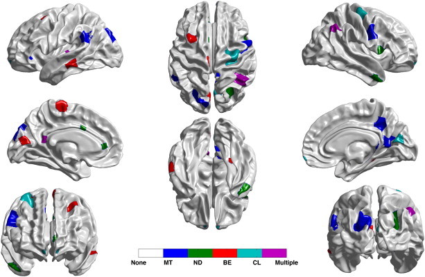
Most discriminative partitions, within each feature set, as determined by the selection frequency from the 100 runs of RHsT. Note that we are only displaying the partitions which were selected at least 25% of the time. Here MT denotes mean thickness, ND denotes nodal degree, BE denotes betweenness centrality and CL denotes clustering coefficient. Those partitions which were selected by more than one feature set are labeled Multiple, and those selected by none of the feature sets as None.
4.1.3. Validation on an independent dataset
The AUC on the validation set compared to the results based on the entire cohort is presented in Table 6. These results show that the performance of our method on validation set (random 50% split of the full cohort) is similar to that on the training set, which demonstrates the robustness of the proposed novel method. Further the trends in AUC across the three classification experiments on the validation set are similar to those on the full cohort.
5. Discussion
In this paper, we have presented a novel ThickNet classifier for differential discrimination between aMCI subtypes and controls. Observing the performance of the ThickNet fusion classifier (in AUC) across the three experiments (Fig. 5), the highest performance is seen in NC vs. md-aMCI (AUC over 0.74). We notice a slightly lower performance in sd-aMCI vs. NC and sd- vs. md-aMCI experiments. This relatively low performance in these two experiments could be due to limited separability i.e. overlap in their cognitive performance, or lack of sensitivity of the proposed method in this experiments. The performance in the two experiments NC vs. md-aMCI and sd- vs. md-aMCI is significantly better than that of NC vs. sd-aMCI experiment (p < 0.05), whereas they do not significantly differ from each other.
Table 4 summarizes the best performance in each experiment, in different performance metrics. We notice that the ThickNet classifier exhibited an AUC of 0.74 in md-aMCI vs NC experiment, demonstrating potential for the detection of md-aMCI. Our classifier displayed better-than-random performance in sd-aMCI vs. NC and sd- vs. md-aMCI experiments. Given that the aMCI is itself an unstable and heterogeneous construct (Brodaty et al., 2013), we do not expect perfect discriminability. In light of these challenges, our results are promising.
Observing the individual weights (Fig. 9), it can be seen that the ThickNet features are contributing to the classifier (non-zero weights), although in varying proportions. The significance of ThickNet features (total weight > 80%) is higher than mean thickness (weight < 15%), supporting the hypothesis that thickness alone does not have adequate discriminatory power. Clustering coefficient is found to have contributed the largest to the discrimination in all the experiments. The contribution of ThickNet features increased with increasing difficulty of the problem, such as NC vs. sd-aMCI and sd-aMCI vs. md-aMCI, which provides further evidence for their utility for the prognostic applications.
5.1. Baseline comparison
In order to better understand the contribution of ThickNet features in improving the predictive power in such challenging problems, we compare the performance of the proposed ThickNet fusion method w.r.t the performance of 1) mean thickness (MT) features alone and 2) combination of MT and hippocampal volumes — see Fig. 10 and Table 5. The results of this comparison show that our novel ThickNet fusion method significantly improved the predictive power (AUC) in detection of md-aMCI, and even more so in already-challenging problems like the NC vs. sd-aMCI and sd- vs. md-aMCI experiments. It is to be noted that different combinations of regional thickness measures have shown potential for the detection of full blown AD (Cuingnet et al., 2011), its performance has been modest in the classification of MCI subtypes (Raamana et al., 2014b).
5.2. Validation on an independent dataset
The classification performance of the ThickNet method on an independent validation set (derived from 50% split of the current cohort) is presented in Table 6. This table shows that the performance of our method on the validation set is similar to the performance on the training set. This shows that performance of the method is robust to unseen data. Compared to the performance obtained from the entire cohort (112 subjects in total), the performance on the validation set (containing only half of the subjects) is showing similar trends across the three experiments. However the validation set performance is lower, which is not unexpected given the small training sample to learn from. Although these results on the validation set demonstrate the robustness of our method, it is always desirable to evaluate our method on an external independent dataset, should a compatible dataset become publicly available in the future.
5.3. Most discriminative partitions
Observing the selection frequency of various partitions in the brain (Fig. 11), we can see that the left lateral temporal region (red region in the top left) is identified as a discriminative region. This region is known to be associated with semantic memory, an area of function that is frequently found disturbed in the prodromal stage of AD and commonly accompanies episodic memory impairment. Moreover, posterior cingulate/medial precuneus region (colored blue) exhibited discriminability as well; and this region is one area that is affected early, both functionally and structurally, in AD as well as MCI. It would be worth further investigating the link between discriminative partitions and structure or function affected in MCI or AD.
It would also be interesting to find any links between these regions and the findings from previous studies of regions with statistically significant group differences. Such a simple comparison of the most discriminative regions identified by our method and the regions with group differences from previous studies reveals a few common regions such as the precuneus and medial temporal lobe.
6. Conclusions
This study contributes to the important discussion of cross-sectional differential discrimination of MCI subtypes. In particular, we have proposed a novel ThickNet classifier to discriminate the subtypes of aMCI, and in particular md-aMCI from NC using baseline cortical thickness features alone. Rigorous analysis of the proposed ThickNet fusion classifier is presented, demonstrating its potential. The ThickNet imaging biomarkers, in combination with biomarkers from other modalities, may assist in identification of patients likely to benefit from therapeutic intervention, or in the future recruitment for clinical trials. A comparison of classification experiments in NC vs. sd-aMCI and sd- vs. md-aMCI is presented as well, to further appreciate the challenges in building a classifier at such an early stage of AD.
Note that this analysis is based on cross-sectional data (at a single time-point), and the diagnosis of MCI (and its subtypes) is based only on baseline assessments, including neuropsychological performance. This baseline clinical diagnosis of MCI is shown to have some instability (Brodaty et al., 2013), which is a pervasive problem with MCI diagnosis as a construct. Hence analysis of patient data, both controls and md-aMCI, with a stable diagnosis would be desirable. There might also be a slight gender imbalance in controls and sd-aMCI groups, which can also be observed in previous studies. In addition, this analysis could be further improved by accounting for the scanner factor during the data pooling stage. Note that there is significant room for improvement of the ThickNet classifier e.g. by applying different (or multiple) kernels for each feature as well as tuning the kernel parameters, as opposed to the current results obtained with a fixed kernel (polynomial kernel, degree = 3). Moreover ThickNet features could be computed using additional measures of centrality, segregation and integration, as well as constructing weighted graphs from the regional links in cortical thickness as opposed to the current choice of binary and undirected graphs in this study.
One of the advantages of this framework is that it is easily extensible i.e. it allows for inclusion of features from other modalities such as Positron Emission Tomography (PET), Diffusion Tensor Imaging (DTI), as well as other morphological and neuropsychological features. Each new feature can be tuned with an additional kernel, which can be easily fused with existing features. Moreover, as the classifier employed is by design multi-class, this method can be readily applied to differential diagnosis e.g. discriminating among NC, sd- and md-aMCI, as well as AD from Frontotemporal disease, or Vascular Dementia etc.
Acknowledgments
We gratefully acknowledge funding support from Alzheimer Society Canada for both P. R. Raamana and M. F. Beg. The authors thank all participants and their supporters in the Sydney Memory and Ageing Study (MAS), and the MAS research team. This study was supported by a National Health and Medical Research Council of Australia Program Grant (no. 350833) and Capacity Building Grant (no. 568940).
Appendix A. Description of quality control on the Sydney MAS cohort
Subjects were excluded from the original MAS cohort (prior to the selection of 112 subjects) owing to their failure in Freesurfer cortical parcellation or in estimation of cortical thickness from our Laplacian streamline method. Our Freesurfer quality control consisted of checking for permanent failure in Freesurfer automatic parcellation, visually examining for accurate Talairach Registration, or when the cortical surfaces have gross errors in following the structural boundaries. Further, even with acceptable Freesurfer parcellation, some subjects were excluded if our thickness computation method based on Laplacian streamlines fails to estimate thickness in either the left or the right hemisphere. We would like to note that none of the 112 subjects being studied in this manuscript presented with major errors in processing, and hence none were excluded.
References
- Alexopoulos P., Grimmer T., Perneczky R., Domes G., Kurz A. Progression to dementia in clinical subtypes of mild cognitive impairment. Dement. Geriatr. Cogn. Disord. 2006;22(1):27–34. doi: 10.1159/000093101. [DOI] [PubMed] [Google Scholar]
- Amieva H., Le Goff M., Millet X., Orgogozo J.M., Pérès K., Barberger Gateau P., Jacqmin Gadda H., Dartigues J.F. Prodromal Alzheimer's disease: successive emergence of the clinical symptoms. Ann. Neurol. 2008;64(5):492–498. doi: 10.1002/ana.21509. [DOI] [PubMed] [Google Scholar]
- Anderson T.M., Sachdev P.S., Brodaty H., Trollor J.N., Andrews G. Effects of sociodemographic and health variables on Mini-Mental State Exam scores in older Australians. Am. J. Geriatr. Psychiatry. 2007;15(6):467–476. doi: 10.1097/JGP.0b013e3180547053. (Jun.) [DOI] [PubMed] [Google Scholar]
- Bäckman L., Jones S., Berger A.-K., Laukka E.J., Small B.J. Multiple cognitive deficits during the transition to Alzheimer's disease. J. Intern. Med. 2004;256(3):195–204. doi: 10.1111/j.1365-2796.2004.01386.x. (Sep.) [DOI] [PubMed] [Google Scholar]
- Beg M.F., Raamana P.R., Barbieri S., Wang L. Comparison of four shape features for detecting hippocampal shape changes in early Alzheimer's. Stat. Methods Med. Res. 2013;22(4):439–462. doi: 10.1177/0962280212448975. [DOI] [PubMed] [Google Scholar]
- Bell-McGinty S., Lopez O.L., Meltzer C.C., Scanlon J.M., Whyte E.M., Dekosky S.T., Becker J.T. Differential cortical atrophy in subgroups of mild cognitive impairment. Arch. Neurol. 2005;62(9):1393–1397. doi: 10.1001/archneur.62.9.1393. (Sep.) [DOI] [PubMed] [Google Scholar]
- Braak H., Braak E. Neuropathological stageing of Alzheimer-related changes. Acta Neuropathol. 1991;82(4):239–259. doi: 10.1007/BF00308809. [DOI] [PubMed] [Google Scholar]
- Braak H., Del Tredici K. The pathological process underlying Alzheimer's disease in individuals under thirty. Acta Neuropathol. 2011;121(2):171–181. doi: 10.1007/s00401-010-0789-4. [DOI] [PubMed] [Google Scholar]
- Brambati S.M., Belleville S., Kergoat M.-J., Chayer C., Gauthier S., Joubert S. Single- and multiple-domain amnestic mild cognitive impairment: two sides of the same coin? Dement. Geriatr. Cogn. Disord. 2009;28(6):541–549. doi: 10.1159/000255240. [DOI] [PubMed] [Google Scholar]
- Brodaty H., Heffernan M., Kochan N.A., Draper B., Trollor J.N., Reppermund S., Slavin M.J., Sachdev P.S. Mild cognitive impairment in a community sample: the Sydney Memory and Ageing Study. Alzheimers Dement. 2013;9(3) doi: 10.1016/j.jalz.2011.11.010. (May, 310–317.e1) [DOI] [PubMed] [Google Scholar]
- Cuingnet R., Gerardin E., Tessieras J., Auzias G., Lehericy S., Habert M.-O., Chupin M., Benali H., Colliot O., Initiative A.D.N. Automatic classification of patients with Alzheimer's disease from structural MRI: a comparison of ten methods using the ADNI database. Neuroimage. 2011;56(2):766–781. doi: 10.1016/j.neuroimage.2010.06.013. (May) [DOI] [PubMed] [Google Scholar]
- Dale A.M., Fischl B., Sereno M.I. Cortical surface-based analysis: I. Segmentation and surface reconstruction. Neuroimage. 1999;9(2):179–194. doi: 10.1006/nimg.1998.0395. [DOI] [PubMed] [Google Scholar]
- Damoulas T., Girolami M.A. Probabilistic multi-class multi-kernel learning: on protein fold recognition and remote homology detection. Bioinformatics. 2008;24(10):1264–1270. doi: 10.1093/bioinformatics/btn112. (May) [DOI] [PubMed] [Google Scholar]
- Eskildsen S.F., Coupé P., García-Lorenzo D., Fonov V., Pruessner J.C., Collins D.L. Prediction of Alzheimer's disease in subjects with mild cognitive impairment from the ADNI cohort using patterns of cortical thinning. Neuroimage. 2013;65:511–521. doi: 10.1016/j.neuroimage.2012.09.058. [DOI] [PMC free article] [PubMed] [Google Scholar]
- Fawcett T. An introduction to ROC analysis. Pattern Recogn. Lett. 2006;27(8):861–874. [Google Scholar]
- Fennema-Notestine C., Hagler D.J., Mcevoy L.K., Fleisher A.S., Wu E.H., Karow D.S., Dale A.M. Structural MRI biomarkers for preclinical and mild Alzheimer's disease. Hum. Brain Mapp. 2009;30(10):3238–3253. doi: 10.1002/hbm.20744. (Oct.) [DOI] [PMC free article] [PubMed] [Google Scholar]
- Fischl B., Sereno M.I., Dale A.M. Cortical surface-based analysis: II: inflation, flattening, and a surface-based coordinate system. Neuroimage. 1999;9(2):195–207. doi: 10.1006/nimg.1998.0396. [DOI] [PubMed] [Google Scholar]
- Fischl B., van der Kouwe A., Destrieux C., Halgren E., Ségonne F., Salat D.H., Busa E., Seidman L.J., Goldstein J., Kennedy D., Caviness V., Makris N., Rosen B., Dale A.M. Automatically parcellating the human cerebral cortex. Cereb. Cortex. 2004;14(1):11–22. doi: 10.1093/cercor/bhg087. (URL http://cercor.oxfordjournals.org/content/14/1/11.abstract) [DOI] [PubMed] [Google Scholar]
- Fitzpatrick M., Sonka M. vol. 2. SPIE-International Society for Optical Engineering; 2000. Handbook of Medical Imaging. (Medical Image Processing & Analysis (PM80)). [Google Scholar]
- Fletcher P.C., Grafton S.T. Repeat after me: replication in clinical neuroimaging is critical. Neuroimage Clin. 2013;2:247. doi: 10.1016/j.nicl.2013.01.007. [DOI] [PMC free article] [PubMed] [Google Scholar]
- Folstein M., Folstein S., McHugh P. Mini-mental state: a practical method for grading the cognitive state of patients for the clinician. J. Psychiatr. Res. 1975;12(3):189–198. doi: 10.1016/0022-3956(75)90026-6. [DOI] [PubMed] [Google Scholar]
- Gibson E., Wang L., Beg M.F. Org Human Brain Mapping, 15th Annual Meeting. 2009. Cortical thickness measurement using Eulerian PDEs and surface-based global topological information. [Google Scholar]
- Hollander M., Wolfe D.A., Chicken E. vol. 751. John Wiley & Sons; 2013. (Nonparametric statistical methods). [Google Scholar]
- Julkunen V., Niskanen E., Koikkalainen J., Herukka S.K., Pihlajamäki M., Hallikainen M., Kivipelto M., Muehlboeck S., Evans A., Vanninen R. Differences in cortical thickness in healthy controls, subjects with mild cognitive impairment, and Alzheimer's disease patients: a longitudinal study. J. Alzheimers Dis. 2010;21(4):1141–1151. doi: 10.3233/jad-2010-100114. [DOI] [PubMed] [Google Scholar]
- Kochan N., Slavin M., Brodaty H., Crawford J., Trollor J., Draper B., Sachdev P. Effect of different impairment criteria on prevalence of “objective” mild cognitive impairment in a community sample. Am. J. Geriatr. Psychiatry. 2010;18(8):711. doi: 10.1097/jgp.0b013e3181d6b6a9. [DOI] [PubMed] [Google Scholar]
- Lee J.K., Lee J.-M., Kim J.S., Kim I.Y., Evans A.C., Kim S.I. A novel quantitative cross-validation of different cortical surface reconstruction algorithms using MRI phantom. Neuroimage. 2006;31(2):572–584. doi: 10.1016/j.neuroimage.2005.12.044. (Jun.) [DOI] [PubMed] [Google Scholar]
- Lerch J.P., Evans A.C. Cortical thickness analysis examined through power analysis and a population simulation. Neuroimage. 2005;24(1):163–173. doi: 10.1016/j.neuroimage.2004.07.045. [DOI] [PubMed] [Google Scholar]
- Liu T., Wen W., Zhu W., Trollor J., Reppermund S., Crawford J., Jin J.S., Luo S., Brodaty H., Sachdev P. The effects of age and sex on cortical sulci in the elderly. Neuroimage. 2010;51(1):19–27. doi: 10.1016/j.neuroimage.2010.02.016. (May) [DOI] [PubMed] [Google Scholar]
- Petersen R.C. Early diagnosis of Alzheimer's disease: is MCI too late? Curr. Alzheimer Res. 2009;6(4):324. doi: 10.2174/156720509788929237. (Aug.) [DOI] [PMC free article] [PubMed] [Google Scholar]
- Raamana P., Weiner M.W., Wang L., Beg M.F. Neurobiology of Aging; 2014. Thickness Network (ThickNet) Features for Prognostic Applications in Dementia. (To Appear) [DOI] [PMC free article] [PubMed] [Google Scholar]
- Raamana P.R., Rosen H., Miller B., Weiner M.W., Wang L., Beg M.F. Three-class differential diagnosis among Alzheimer disease, frontotemporal dementia and controls. Front. Neurol. 2014;5(71) doi: 10.3389/fneur.2014.00071. URL http://www.frontiersin.org/brain_imaging_methods/10.3389/fneur.2014.00071/abstract. [DOI] [PMC free article] [PubMed] [Google Scholar]
- Raamana P.R., Wang L., Beg M.F. Proceedings of MICCAI Machine Learning in Medical Imaging Workshop. Vol. 8184. Springer-Verlag; 2013. Thickness network (ThickNet) features for the detection of prodromal ad; pp. 115–123. (LNCS). [Google Scholar]
- Raamana P.R., Wen W., Kochan N.A., Brodaty H., Sachdev P.S., Wang L., Beg M.F. The sub-classification of amnestic mild cognitive impairment using mri-based cortical thickness measures. Front. Neurol. 2014;5(76) doi: 10.3389/fneur.2014.00076. (URL http://www.frontiersin.org/neurodegeneration/10.3389/fneur.2014.00076/abstract) [DOI] [PMC free article] [PubMed] [Google Scholar]
- Rubinov M., Sporns O. Complex network measures of brain connectivity: uses and interpretations. Neuroimage. 2010;52(3):1059–1069. doi: 10.1016/j.neuroimage.2009.10.003. [DOI] [PubMed] [Google Scholar]
- Sachdev P.S., Brodaty H., Reppermund S., Kochan N.A., Trollor J.N., Draper B., Slavin M.J., Crawford J., Kang K., Broe G.A., Mather K.A., Lux O. The Sydney Memory and Ageing Study (MAS): methodology and baseline medical and neuropsychiatric characteristics of an elderly epidemiological non-demented cohort of Australians aged 70–90 years. Int. Psychogeriatr. 2010;22(08):1248–1264. doi: 10.1017/S1041610210001067. (Dec.) [DOI] [PubMed] [Google Scholar]
- Seo S., Im K., Lee J., Kim Y., Kim S., Kim S., Yang D., Kim S., Cho Y., Na D. Cortical thickness in single-versus multiple-domain amnestic mild cognitive impairment. Neuroimage. 2007;36(2):289–297. doi: 10.1016/j.neuroimage.2007.02.042. [DOI] [PubMed] [Google Scholar]
- Stonnington C.M., Tan G., Klöppel S., Chu C., Draganski B., Jack C.R., Jr., Chen K., Ashburner J., Frackowiak R.S.J. Interpreting scan data acquired from multiple scanners: a study with Alzheimer's disease. Neuroimage. 2008;39(3):1180–1185. doi: 10.1016/j.neuroimage.2007.09.066. (Feb.) [DOI] [PMC free article] [PubMed] [Google Scholar]
- Wallace B.C., Small K., Brodley C.E., Wang L. Data Mining (ICDM) 2011. Class imbalance, redux. [Google Scholar]
- Whitwell J., Petersen R., Negash S. Patterns of atrophy differ among specific subtypes of mild cognitive impairment. Arch. Neurol. 2007;1–9 doi: 10.1001/archneur.64.8.1130. [DOI] [PMC free article] [PubMed] [Google Scholar]
- Witten I.H., Frank E. Morgan Kaufmann; 2005. Data Mining: Practical Machine Learning Tools and Techniques. [Google Scholar]
- Yaffe K., Petersen R.C., Lindquist K., Kramer J., Miller B. Subtype of mild cognitive impairment and progression to dementia and death. Dement. Geriatr. Cogn. Disord. 2006;22(4):312–319. doi: 10.1159/000095427. [DOI] [PubMed] [Google Scholar]
- Yezzi A.J.J.L.P. An Eulerian PDE approach for computing tissue thickness. IEEE Trans. Med. Imaging. 2003;22(10) doi: 10.1109/TMI.2003.817775. [DOI] [PubMed] [Google Scholar]


