Fig. 3.

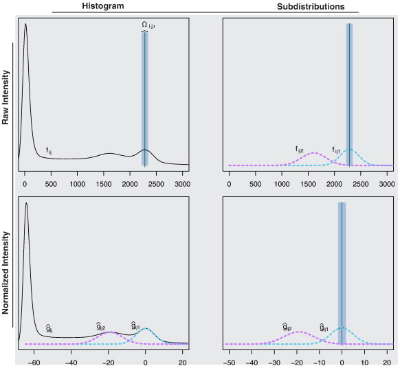
Example of the white stripe normalization procedure. In the top left plot, the raw histogram of a T1-w image is shown. Using a peak-finding algorithm, μ_ij1^∗ and thus Ω_i,j,τ are estimated. In the right column of the figure, Ω_i,j,τ is shown before and after normalization. The density of the intensities in NAWM before (f_ij1) and after normalization $\left({\displaystyle {\widehat{g}}_{\mathit{ij}2}}\right)$ is shown using dashed magenta lines. The bottom left plot shows the histogram after white stripe normalization.