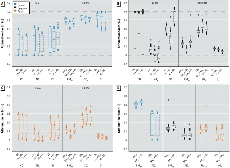
Figure 4.

Attenuation of model coefficients in a classical-error, single-pollutant framework and in bipollutant models, assuming that one pollutant has an effect and one pollutant has no effect. (A) λ for local–local and regional–regional pollutant pairs due to δ_spatial. (B) λ local–local and regional–regional pollutant pairs due to δ_population. (C) λ for local–local and regional–regional pollutant pairs due to δ_total. (D) λ due to δ_spatial, δ_population, and δ_total for a local–regional pollutant example (i.e., PM_2.5, PM_2.5 and No_x). See Supplemental Material, Figure S5, for all local–regional pollutant pairs. The bottoms and tops of boxes represent 25th and 75th percentiles, lines within boxes indicate the median, and the whiskers represent 5th and 95th percentiles; n = 193. Solid-line boxes indicate attenuation factors for single-pollutant models, and dashed-line boxes represent attenuation factors for bipollutant models. The top row of x-axis labels indicates the pollutant effect being considered (e.g., CO), and the bottom row of x-axis labels indicates the relevant model and the presence or absence of co-pollutants (e.g., CO, CO + NO_x, CO + EC). For example, for the three plots representing attenuation factors for CO, the first plot is the set of attenuation factors for CO in a single-pollutant model; the second is the attenuation factors for CO in a bipollutant model with NO_x, assuming that NO_x has no effect; and the ^third is the attenuation factors for CO in a bipollutant model with EC, assuming that EC has no effect. λ = 1 indicates no attenuation, λ = 0 indicates null results.