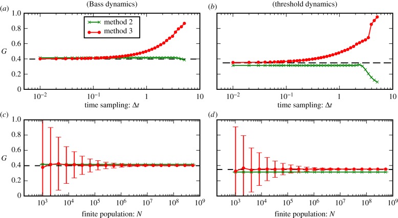
Figure 5.

Method 2 is more robust against perturbations than Method 3. Estimation of G in undersampled versions of the time series used in figure 2 for Bass (left) and threshold (right) dynamics. The true G [equation (2.5)] is shown as a dashed line and Methods 2 and 3 are shown by symbols. (a,b) Undersampling in time: achieved by varying the time-resolution Δt of the time series, i.e. we sample ρ(t) at times . Resolution increases for Δt → 0. (c,d) Undersampling of the population N. The surrogate time-series ρ(t) in figure 2 assume N → ∞. We consider time series for which only a finite population N is observed. The observed fraction of adopters is determined from N independent Bernoulli trials with probability ρ(t). This corresponds to adding noise to each data point ρ(t). Resolution increases for N → ∞. For each N, we plot the average and standard deviation of G computed over 1000 trials. (Online version in colour.)