Abstract
Attractant-based trap networks are important elements of invasive insect detection, pest control, and basic research programs. We present a landscape-level, spatially explicit model of trap networks, focused on detection, that incorporates variable attractiveness of traps and a movement model for insect dispersion. We describe the model and validate its behavior using field trap data on networks targeting two species, Ceratitis capitata and Anoplophora glabripennis. Our model will assist efforts to optimize trap networks by 1) introducing an accessible and realistic mathematical characterization of the operation of a single trap that lends itself easily to parametrization via field experiments and 2) allowing direct quantification and comparison of sensitivity between trap networks. Results from the two case studies indicate that the relationship between number of traps and their spatial distribution and capture probability under the model is qualitatively dependent on the attractiveness of the traps, a result with important practical consequences.
Trap networks are crucial components of many pest detection, delimitation, control, Integrated Pest Management, and eradication programs1,2. For many insect pests, traps consist of a semiochemical or food-based attractant (lure), sometimes in combination with a pesticide and/or adhesive. Examples of attractant-based trap networks include the approximately 30,000-trap Ceratitis capitata (medfly) detection network in Southern California, USA3, a high-density trapping program for eradication of Lymantria dispar (Asian Gypsy moth) in New Zealand4, and a delimitation network for Popillia japonica (Japanese Beetle) in Missouri, USA5.
An important practical issue inherent to trapping, regardless of the goal, is where to place traps. The most common approach is trap deployment in a grid of cells: a feasable trap density is determined (in the case of medfly detection in California, for example, 5 traps per square mile), and then traps are set within each cell in sites believed most likely to result in catches of an invading or established pest. Research studies are used to determine optimal habitat types for trap placement6, but other times such results are not available, and expert judgement is used to determine placement3.
Since trap networks are expensive to set up and maintain, particularly over large areas, research focuses on the question of appropriate trap densities to be used in each cell for different purposes. In a detection network, for example, the density per cell may vary depending on habitat suitability for the pest in question or the attractiveness of the lure used3. Due to the importance and cost of trap networks, their spatial optimization has received increasing attention in recent years7,8; spatial placement of traps can also benefit from models focused on the question of placement.
Mathematical or computer models of insect traps can be classified into two groups9: 1) those that model an area or volume within which receptive insects are captured, exemplified by the Effective Attraction Range (EAR)10, which relates the captures in an unbaited passive trap with those in a baited trap to calculate the physical size an unbaited trap would need to be in order to catch as many insects as the baited version. The area- or volume-based approaches include earlier concepts, such as the Active Space11,12,13 and Attraction Range14,15. 2) Models that focus on capture probability based on the distance of an individual insect from the trap being modeled. A recent example of a capture probability based model16 considers both the distance from the trap and dose of attractive lure to determine a probability of insect capture. For the effect of distance, Branco et al16 use a logistic equation; other capture probability models employ exponential17,18 or Cauchy19 distributions for this purpose.
In this paper we present a novel capture probability model of trap attraction based on distance from a trap and the hyperbolic secant function. The model as used here is primarily focused on the sensitivity of detection networks of traps, but it can be easily extended to other purposes such as delimitation or control. We explicitly consider the attractiveness of the lure used in the trap, the spatial relationship between the insect and the trap, the movement of insects, and the ecology of the area. We describe the mathematical basis of our trap model, validate its behavior using field data on trap networks, use a computational approach to place modeled traps into a variable landscape, and examine the effectiveness of trapping networks.
Our model is useful for optimizing trap placement to minimize program operating costs and comparing the sensitivity of networks with varying densities or placements. It allows consideration of a heterogeneous landscape in two ways: 1) by permitting per-trap attraction to vary depending on the habitat at the site of each trap and 2) by incorporating a risk map of where outbreaks or insect densities are likely to be highest. The model can be used to rigorously estimate the probability of insects existing in the area when none are captured, a topic of considerable ecological, economic and regulatory importance20,21.
Results
Modeling overview
The principal model we describe aims to answer two questions about a given trapping network: 1) what is the average detection ability of the trapping network and 2) what is the average probability of an insect being caught in a trap over time? If we can calculate these variables for a variety of situations, then we can apply this information to the specific goals of a trapping network, be they detection, delimitation or quantification. The model developed requires knowledge of certain key parameters, including the position and range of attraction of given trap and lure combinations and the movement parameters of the target insect(s). Extension of our model to questions beyond detection may require information on the species' developmental, life history and demographic characteristics.
Two models are examined here in the context of the sensitivity of a trapping network. The first, termed “Area-Based”, is the Effective Attractive Radius, circular (EARc) of Byers, which is defined as the radius around a baited trap within which all insects that enter are captured22. The EARc model is used to introduce important concepts for the second model, upon which we focus most of our attention.
The second modeling approach, which is capture probability- based, models the probability of an insect detecting the baited trap and initiating a behavioral sequence that results in its capture as a function of its distance from the trap. We present a previously unused mathematical function for relating distance to probability of capture, the hyperbolic secant, which has some desirable properties in terms of field estimation. We also apply the new function in a grid to explore the effects of trap attractiveness and positioning on network sensitivity. We give practical details on the implementation of our capture probability model in the Methods section.
Area-based Approach
We can relate insect capture probability to the ratio of the sum of capture areas of a set of traps (total combined area where there is a 100% chance of capture, which we denote Ac) to the overall available area (A). Assume we have an m × n grid of traps (m and n are the number of traps in each direction) evenly spaced a distance s meters apart in both dimensions. This setup is shown graphically in Figure 1, which shows a 4 × 3 array of traps.
Figure 1. Idealized representation of a trapping grid.
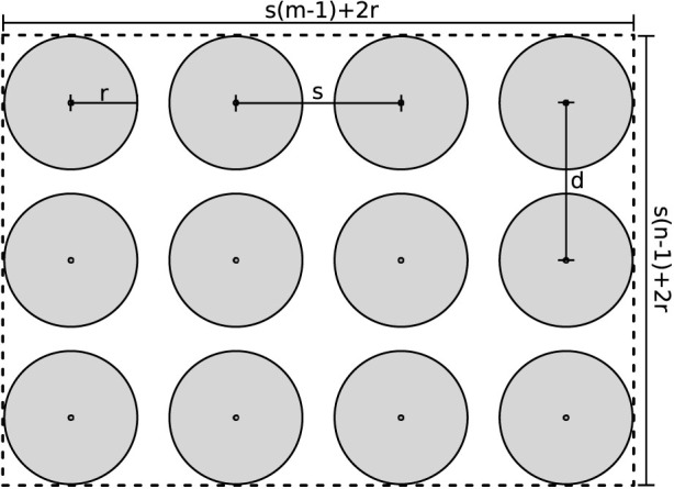
Each trap has a capture radius r. This defines an area around the trap within which an insect will be captured with probability = 1. We can calculate the total area of the trap capture radii as
 |
when 2r < s. We can define the overall grid area as
 |
From this simple model we can define a instantaneous capture probability, p = Ac/A, which is equivalent to the probability of a randomly chosen point being within the capture radius of a trap. Figure 2 shows how p changes with increasing trap attractiveness (r). Values are chosen to represent, approximately, a regular 8 × 8 grid with 150 m spacing, the trapping network in South Australia for medfly with a trap about every 400 m (6.25 traps per km2, which translates to a trap every 400 m in a grid) and approximately the density of the trapping network in Southern California also aimed at medfly, with a trap every 800 m (5 traps per mi2 = 1.93 traps per km2, a trap every 720 m)23.
Figure 2. Changes in the probability of capture p of an individual with increasing trap attraction (r = area within which there is a 100% chance of capturing a fly) and varying grid density (represented by inter-trap spacing, s) in an approximately 2.6 km2 area (1 mi2).
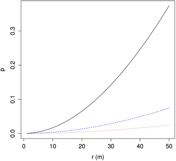
Solid line: 10 × 10 grid of traps with s = 150 m; broken line: 4 × 4 grid with s = 400 m; dotted line: 3 × 3 grid with s = 800 m.
Capture Probability Model
One important way in which the area-based approach presented above is unrealistic is that the probability of capture for an individual with distance from a trap has only two values (0 or 1). In a capture probability models, the probability of an individual insect being caught in a trap can take a wider variety of values depending on its distance from the trap (d). In this way, the capture arena becomes three-dimensional, with points represented by (x, y, p), where x, y are positions in space and p is capture probability, which may take any value between 0 and 1.
We calculate the distance to a trap as  , where (xt, yt) is the position of the trap, and (x, y) is the position of the insect. For d ≥ 0, we use an exponential decay with a logistic (H(2λd)) to model the probability of being captured:
 |
where
 |
these can be combined into a simpler form as
 |
which is sech(λd), where sech is the hyperbolic secant function. Figure 3 shows how the probability of capture changes with distance from the trap given λ. The parameter λ is the “attractiveness” of the trap, with smaller values representing a more attractive trap. The sech function is mathematically related to the exponential and logistic functions used in previous research17,18,19. In our model, sech produces a probability; the value of the function when λd = 0 is 1, and the limit as λd approaches infinity is zero.
Figure 3. Capture probability for an individual insect versus distance from a trap, where probabilities were calculated via equation 5 for 1/λ = 10 (black), 30 (blue) and 50 (red) meters.
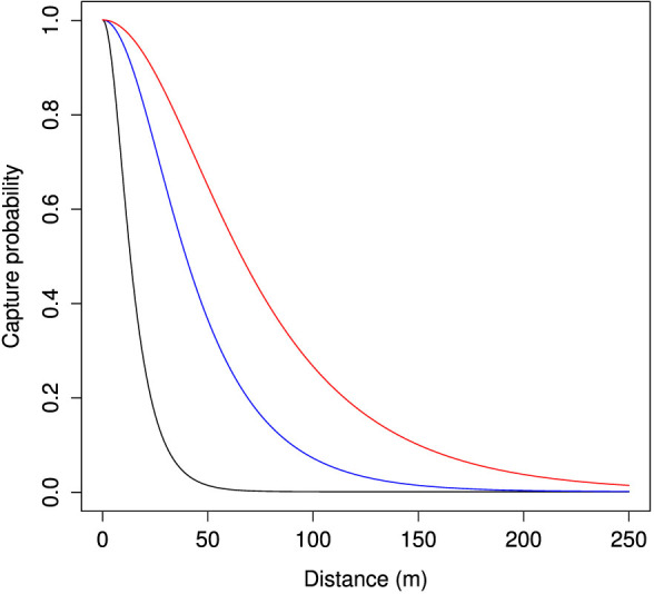
1/λ = represents the distance, in meters, where we expect about 0.65 probability of capture.
There are two useful properties of this function that allow us to relate it to measurements that might be made on actual insects. The first is that f(0, λ) = 2/2 = 1. This means that the probability of capture at distance 0 = 1 regardless of λ. The second useful feature is that f(1/λ, λ) = 0.6481 for any positive λ. This constant means that 1/λ is equal to the distance at which there is an ≈ 65% probability of an insect being caught by a trap, a concept that has a simple meaning and can allow easy comparison of trap attraction across lures and species.
Instantaneous Capture Probability
Considering a trap with attractiveness λ at distance dx,y from a given point (x, y) in a grid with area A encompassing x0 < x < xm and y0 < y < ym, the average instantaneous capture probability across the entire grid is given by:
 |
The situation with multiple traps is more complicated, as capture by one trap is not independent of capture by another trap. So instead we consider the probability of escape. Given an insect at point (x, y) and n traps with each trap t having distance dx,y,t from the insect, the total instantaneous probability of escape is:
 |
From 6 and 7, we derive the following formula to calculate the average instantaneous probability across a grid with n traps:
 |
with  . Figure 4 shows results from our capture probability model for a variety of trapping grids with varying trap strengths.
Figure 4. Changes in the average instantaneous probability of capture  with increasing trap attraction (1/λ = distance at which there is a 65% chance of capturing a fly) and varying grid density (represented by inter-trap spacing, s) Solid line: 8 × 8 grid of traps with s = 75 m; broken line: 8 × 8 grid of traps with s = 150 m; dotted line: 4 × 4 grid with s = 400 m; dashed-dotted line: 3 × 3 grid with s = 800 m.
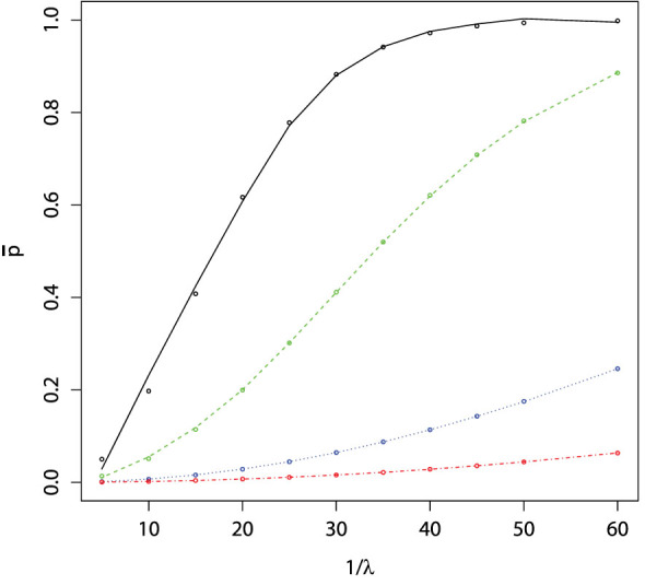
The value  represents the average instantaneous probability of being captured for a given arena, number of traps and attractiveness of the traps. In a heterogeneous environment, traps containing the same lure may not be equally attractive; this situation can be accommodated using equation 8. It is important to stress that this outcome does not yet take into account time- it is only the average probability of being captured given appearance in a random position within a given arena.
Probability of Capture Over Time
We now consider how the probability of detecting a population of insects changes over time. We use a diffusion model to simulate insect locations. This model specifies the position of individuals moving randomly in a two-dimensional plane after a given amount of time24,25
 |
where N is the population density, T is time (in days), x, y are spatial coordinates (in meters) and D is the diffusion coefficient (m2 per day)25. Over an infinite plane, the solution to the above equation produces a bivariate normal distribution of density as a function of the diffusion coefficient and time. The probability density function (pdf) of this distribution is a common starting point for modeling population spread over time:
 |
In the above, σ is the standard deviation, this assumes that μ = 0,  and σx = σy = σ and that cor(x, y) = 0. We omit the reaction terms often seen in diffusion models to consider demography because we focus on modeling the relatively short time periods involved in detection26. The absence of boundary conditions in our diffusion model means that insects may travel outside the trap grid area as defined in the instantanious estimate of detection probability (
 ). When this occurrs, the probability of detecting insects in those positions effectively becomes zero.
We are thus able to obtain a distribution of a population of insects at a particular time step given an initial population location (the mean), D and the amount of elapsed time (represented in the variance, σ). By using this pdf it is possible then to obtain insect positions and then, for each position, calculate the probability of capture (using a version of eq. 7 for a single position). The capture probability of the individuals in the population can be examined over time to allow the comparisons in the following sections.
Example: Medfly detection array in Southern California
Ceratitis capitata is a major threat to agriculture around the world, because it infests a large variety of commercial fruit crops27 and persists in a wide variety of habitats28. The first detection of medfly in California occurred in 1975, and it has regularly reoccurred since the early 1980s7. The movement of medfly is generally considered to be reasonably well modeled by a diffusion process and is thought to be quite extensive, with D estimated to be near 1 × 10⁵ m2/day29.
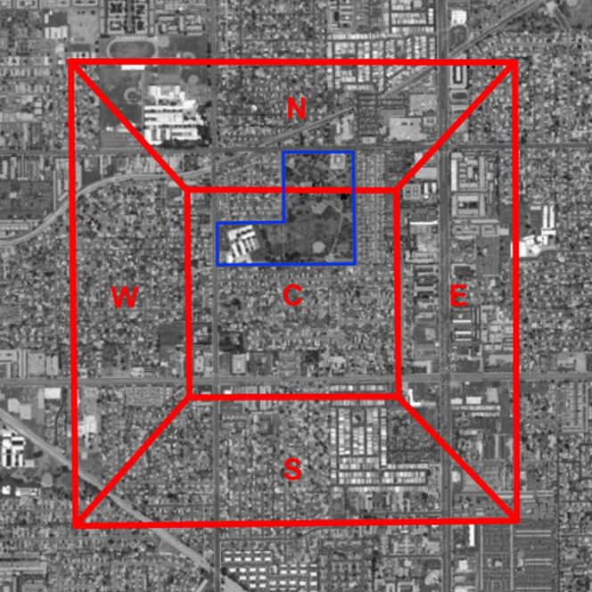
The current standard detection network in the Los Angeles basin for medfly consists of a trap density of five Trimedlure baited Jackson traps plus an additional five protein lure-baited McPhail traps per square mile3. These traps are evenly distributed by dividing each square mile into quintiles and placing one Trimedlure and one protein lure trap on a tree (preferably a host) within each quintile. Traps are checked every 14 days, and locations rotated within the quintile every 6 weeks. The map in Figure 5 is an example of a single square mile of the trapping network in Anaheim, California.
Figure 5. A single square mile of the trapping grid in Anaheim, CA.
Each square mile is divided into five quintiles (N,S,E,W and C). One trap is placed per quintile, its position changed every six weeks. The park on the E-W border between the C and N quintiles is the one assumed to be high-risk in the main text. Source: Esri, DigitalGlobe, GeoEye, i-cubed, USDA, USGS, AEX, Getmapping, Aerogrid, IGN, IGP, swisstopo and the GIS User Community.
When C. capitata are found in one of the traps, there are usually quarantine, eradication, and phytosanitary measures implemented to eliminate the medfly from the infested area3. One of the important measures undertaken is that the trap density is increased considerably in the area where medflies are detected. In the “core” area, a 1 square mile region around an outbreak, the number of traps is increased to 100. In a buffer area one mile out from the core area, trap density is increased to 50 Trimedlure-baited Jackson traps per square mile.
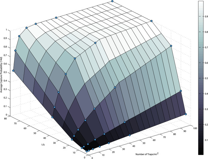
Figure 6 shows changes in the average capture probability for a single individual medfly as the number of traps per square mile and the attractiveness (driven by use of different lures, for example) of the traps are varied. For traps with low attractiveness there is only a modest increase in the average capture probability with increasing trap number; a larger increase in average capture probability is seen with increasing trap attraction.
Figure 6. Changes in the average capture probability after two weeks of individual medfly (or other insect) in a one square mile arena resulting from variation in the number of traps and in the attractiveness of each trap.
Points represent means of 250 simulations of 300 insects each with random outbreak locations and D = 10,000 m2/day29.
A second question of interest regarding medfly trap networks is the effect of risk information on estimates of detection probability. For the capture probability-based models the effect of varying risk of outbreaks can be incorporated by selecting population positions to correspond to risk rather than surveying a random set of locations. Under a scenario where the park indicated in the caption of Figure 5 is an area of higher risk for outbreaks, we compared the average capture probabilities of simulations centered at that location with a spread around it with random outbreak locations.
Comparison of random outbreak locations with risk-based based outbreak locations show that if the risk is highly concentrated in one area the variance in the estimate of average capture probability can be significantly reduced (Figure 7). However, if the risk is diffuse over a large area the variance can be greater than having random outbreak locations within a defined arena. Figure 7 also includes the instantaneous capture probability raised to n, where n is the number of days for comparison with the diffusion-based capture probability over time approach. The mean values are similar, but the diffusion-based approach has the advantage of providing a variance for the mean estimate.
Figure 7. Comparison of random and risk-map based outbreaks for a single square mile of a medfly trapping network in Anaheim, CA.
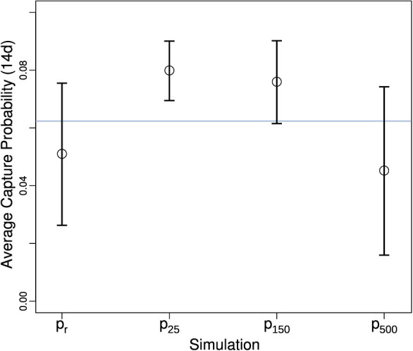
Bars show mean values, and whiskers indicate SD.  is the instantaneous estimate raised to the 14th power, indicated by the grey horizontal line; pr is the movement-based estimate with random outbreak locations; px indicate the probability of capture when outbreak locations are normally distributed and centered at the park (see Fig. 5) with x indicating the variance in outbreak location in meters.
Example: Asian Long-horned Beetle in Massachusetts
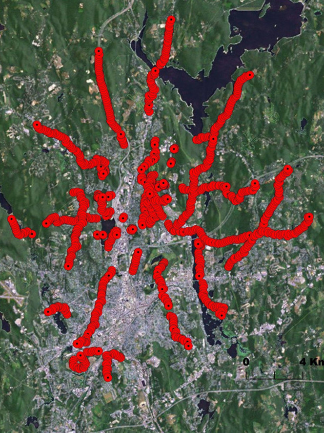
The Asian longhorned beetle, A. glabripennis (ALB), is an exotic wood-boring beetle native to China and Korea. It has been a frequent problem as an invasive in North America, with discoveries in many major cities, including, but not limited, to New York City, Chicago, Toronto, and Boston, from 1996 to the present day30. One of the largest outbreaks was discovered in 2008 in Worcester, MA, generating a quarantine zone of 285 square kilometers31. Extensive attempts at eradication in this zone have been attempted, with over 30,000 trees being removed31. To compliment this eradication effort, the utility of establishing a trapping network is being evaluated. Several plant volatile blends and ALB produced pheromones are promising for use in survey and detection grids32,33,34. While laboratory and field experiments demonstrate ALB response to the lures, yielding an increased trapping rate observed in lured traps compared to controls, quantitative knowledge of the attractiveness of the traps is not known. In addition, the type and location of the trap used can influence trap catches and effectiveness35,32. In the case of the Worcester trapping network, linear trapping transects were employed, radiating from the infestation epicenter and following major corridors to allow for accessibility of traps and ease of trap placement (Fig. 8). This is in contrast to the gridded network used in medfly survey, where distances between traps are roughly uniform, but trap servicing may require additional labor and time.
Figure 8. Trap locations in a 1,013 trap network for ALB in Massachusetts.
Source: Esri, DigitalGlobe, GeoEye, i-cubed, USDA, USGS, AEX, Getmapping, Aerogrid, IGN, IGP, swisstopo and the GIS User Community.
Movement of ALB is quite different from that of medfly. ALB has a one-year life cycle, a large percentage its lifetime is spent within the host tree, and adult emergence and flight period occurs over only a few months of the year. Field experiments in the native range in China demonstrated estimated ALB median flight distance at 20–30 m per day, although the movement is random in terms of direction. Due the randomness of movement direction, dispersal distance may be as little as 100 m per life-time (with a one year life cycle), with some estimates generating a mean dispersal in the hundreds of meters36. This distance can vary, and mark-release-recapture experiments demonstrate that gravid females may disperse as far 2,644 m36,37. In addition, dispersal is density-dependent, with greater movement probability existing when the density of beetles at a location is high38. In a low density infestation, re-infestation of the parent tree is more likely than long-range dispersal and movement to a new host (R. Trotter, pers. comm.). Phenology of outbreaks corresponds to dispersal estimates from mark-release-recapture studies, with a 130 m average distance between ALB infested trees in Worcester31. This corroborates life-time dispersal distances estimated from these studies. Utilizing these estimates, the influence of the linear trap array network versus even spacing of the trap array across the entire network can be considerd.
Figure 8 shows the trapping network for ALB around Worcester (see39 for more details). We compared the capture probability of this grid under two levels of attractiveness with a regular array of a similar number of traps over the same area. The comparison (Table 1) shows that the real grid under low attraction has an approximately 4% average cumulative capture probability after 30 days and that the capture probability is roughly doubled when the traps are arranged in a regular grid. For the high attractiveness scenario, however, the average cumulative capture probability is approximately tripled by placing the traps in a regular grid (Table 1).
Table 1. Average cumulative individual capture probability after 30 days for the real ALB trapping network compared with a regular (32 × 32) grid at two levels of attraction (1/λ).
| Layout | (1/λ) | Mean capture p (SD) |
|---|---|---|
| Real | 10 | 0.04 (0.17) |
| Grid | 10 | 0.08 (0.19) |
| Real | 35 | 0.12 (0.31) |
| Grid | 35 | 0.34 (0.35) |
Discussion
The sensitivity of a trapping network as measured by capture probability is a topic of critical importance to pest detection, delimitation, and eradication. Our model can improve efforts to optimize trap networks in two important ways: 1) it introduces an accessible and realistic mathematical characterization of the operation of a single trap that lends itself easily to parametrization via field experiments, and 2) it allows direct quantification and comparison of sensitivity between trap networks. In addition to these two contributions, the simulation results presented above for the two case studies indicate that the relationship between number of traps in a network and capture probability is highly dependent on the attractiveness of the traps, a result with important practical consequences.
The hyperbolic secant capture probability model has the useful property of requiring a single parameter, λ, that defines the attractiveness of the trap. The reciprocal of this parameter is a constant, which translates to the distance at which there is a 65% probability of capture. This contrasts with logarithmic and exponential capture probability models as previously employed, which require two parameters, may have undefined capture probabilities at distance 0 or do not have easily understood real-world translations.
Another useful property of our capture probability model is that experimental designs to estimate λ for real traps are immediately obvious, especially in the case of fruit flies. Previous studies with medflies have used a centrally located trap and counted numbers of marked flies released at different distances40,41 and this approach could be repeated for estimating λ if the proportion of responsive flies were taken into account in the calculation of p. Another approach is to create a grid of traps, release a known number of marked individuals in the network and check for the proportion receptive flies recaptured42. From this proportion and the relationship between λ and capture probability (see Figure 4), it is possible to estimate trap attractiveness in diverse ecological settings. Work is ongoing in Hawaii to develop the parameter λ for economically important Tephritids and the traps used to detect and monitor them.
Previous work has allowed direct comparison of the attractiveness of different traps, particularly the EAR and EARc of Byers and colleagues10,22. This crucial development allows comparisons of trapping networks, though it is less realistic for how insects are attracted to traps compared with capture probability-based approaches. Experimental designs to parametrize EAR-based models also usually depend on captures of insects with passive traps, which is better suited for insect species that are active fliers and in higher densities. The capture probability based model here offers an alternative method for characterizing capture probability in space that may be more realistic for many insects.
One important result from the case studies is that the effect of increasing trap numbers is highly dependent on the attractiveness of the traps. If the trap has low attractiveness, increasing the number yields a roughly linear and often quite shallow increase in the capture probability for the entire network. However, if each trap has high attractiveness, then increasing the number yields a very quick increase in average capture probability to an asymptote around 1 (Figure 6). This suggests that investment in development and deployment of a more highly attractive lures, such as α-copaene43 or ceralure44 in the case of medfly, will be more effective than increasing the number of traps containing a lure with low attraction.
A second important consequence of the relationship between number of traps per unit area and capture probability is that there is an optimum number of traps for a given landscape, above which little benefit will accrue to the network operator in terms of capture probability. Cost-benefit analysis can be applied in conjunction with this model to determine the opimal number and placement of high attraction traps. In addition, alternative detection methods may actually outperform mass trapping if the trap attractiveness is low. For example, in ALB surveys, alternative methods include manual surveys of host trees for oviposition sites, larval frass, and adult exit holes either from the ground or using tree climbers30. While the labor cost of performing surveys is high, detection using this method may be more sensitive then trapping. These are complex problems, with no clear solution, but better ability to model trapping efficiency can have a clear benefit.
A third practical consequence of the simulation results above relates to the deployment of traps along roads versus in a regular grid (e.g.45) The ALB case presented shows that the actual capture probability of linear trapping networks could be compared with gridded or other arrays, ensuring that the comparison is valid. The impact of an actual trap grid can be compared quantitatively with an idealized grid.
The modeling approach presented here is flexible and could be made more specific for particular insects or trapping goals. It is similar in spirit to another recent model26, which was motivated by the spread of Bactrocera fruit flies in Africa. Dufourd and colleagues examine the question of trap placement optimization, an important practical question that the current study could also inform.
The movement of insects over the landscape is clearly an area where our model could be made more realistic. The computer code we used for the simulations in this study includes an alternative movement model, the random correlated walk46,47 (see Methods). While this mode is more realistic, it requires additional parameters (mean step size, turning angles and steps per unit time), which have yet to be developed for most insects. We note that the assumption of random diffusion is weak for the ALB case presented, as this insect has dispersal behavior that is affected by host status and is characterized by distributional patchiness. For this insect, the alternative simulation of dispersal would be useful, perhaps combined with a time-varying movement rate.
Future work to develop this model could also include a function to vary λ as lures used in traps age. Again, the model is flexible enough to easily accomodate such an enhancement. We also expect that this model will serve as a basis for spatially explicit agent-based models of insect pest populations48,49,50.
Methods
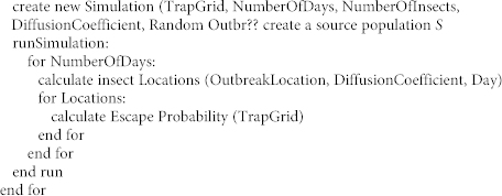
The software implementation of the trap grid model named “TrapGrid” is available for download at http://brianreallymany.github.io/TrapGrid/. This program generates two outputs. The first is the average instantaneous escape probability for an entire grid. This value is dependent only on the placement and attractiveness of the traps in the grid. The second quantity output is the cumulative escape probability of a grid over a given time period. This value depends on the characteristics of the grid, and also on the location of a simulated outbreak and the quantity and diffusion coefficient of the insects.
As noted in equation 8, the calculation of the average capture probability within a given area involves double integration of the product of several single-trap capture probability formulae. This product of formulas is a nonelementary integral. We choose, therefore, to estimate this quantity using Monte Carlo approximation. Within the boundaries of a grid, we randomly choose a pair of coordinates and calculate the escape probability from this point. We repeat this step with a large number of randomly-chosen points, then average their escape probabilities. The entire process is then repeated with a new, larger set of points, and the two average escape probabilities are compared. If they are within a user-determined tolerance of each other, the last probability is considered accurate. If not, the process continues, each time comparing the two most recent averages.
Calculating the cumulative escape probability of a grid over time involves more parameters. TrapGrid approaches the problem by executing a given number of simulations with similar parameters and randomized outbreak locations in order to obtain a distribution of cumulative escape probabilities within a certain time limit.
User-defined parameters include the layout of traps (TrapGrid), NumberOfDays to run each simulation, NumberOfInsects per outbreak, DiffusionCoefficient for the insects, and NumberOfSimulations to run. Below is a brief algorithm of the simulation.
for NumberOfSimulations:
 |
Author Contributions
N.C.M. concieved and developed the model, wrote the main text and produced the figures. B.H. assisted with model development, programmed the main simulation software and wrote the “Methods” section. S.M.G. assisted with model development, contributed to the main text and wrote the section “Example: Asian Long-horned Beetle in Massachusetts”.
Acknowledgments
We thank John Byers for inspiration and early input on this computer model. Thanks also to Robert Trotter for the ALB trap data and to Julie Gaertner for assistance with maps. This work was funded by the United States Department of Agriculture-Agricultural Research Service (USDA- ARS) and B.H. was supported by funding through USDA Farm Bill project 3.0251. Opinions, findings, conclusions, or recommendations expressed in this publication are those of the authors and do not necessarily reflect the views of the USDA. USDA is an equal opportunity provider and employer.
References
- Apple, J. & Smith, R. (eds.) Integrated pest management (Plenum, New York, 1976). [Google Scholar]
- El-Sayed A. M., Suckling D. M., Wearing C. H. & Byers J. A. Potential of mass trapping for long-term pest management and eradication of invasive species. J. Econ. Entomol. 99, 1550–1564 (2006). [DOI] [PubMed] [Google Scholar]
- Gilbert A., Bingham R., Nicolas M. & Clark R. Insect trapping guide, 12th edition (CDFA, Sacramento CA, 2010). [Google Scholar]
- Gray D. R. Hitchhikers on trade routes: A phenology model estimates the probabilities of gypsy moth introduction and establishment. Ecol. Appl. 20, 2300–2309 (2010). [DOI] [PubMed] [Google Scholar]
- Denning J. & Goff C. Eleven years of Japanese beetle control in Missouri- 1934–1944. Mo. Dept. Agric. Bull. 42, 1–17 (1944). [Google Scholar]
- Bakke A. Deploying pheromone-baited traps for monitoring Ips typographus populations. Z. Angew. Entomol. 99, 3339 (1985). [Google Scholar]
- Papadopoulos N. T., Katsoyannos B. I. & Nestle D. Spatial autocorrelation analysis of a Ceratitis capitata (Diptera: Tephritidae) adult population in a mixed deciduous fruit orchard in northern Greece. Environ. Entomol. 32, 319–326 (2003). [Google Scholar]
- Lyons D. B., Sanders C. J. & Jones G. C. The use of geostatistics and GIS as tools for analyzing pheromone trap data at a landscape level: an update. IOBC/WPRS Bull. 25, 157–166 (2002). [Google Scholar]
- Byers J. A. Active space of pheromone plume and its relationship to effective attraction radius in applied models. J. Chem. Ecol. 34, 1134–1145 (2008). [DOI] [PubMed] [Google Scholar]
- Byers J. A., Anderbrant O. & Löqvist J. Effective attraction radius: A method for comparing species attractants and determining densities of flying insects. J. Chem. Ecol. 15, 749–765 (1989). [DOI] [PubMed] [Google Scholar]
- Bossert W. H. & Wilson E. O. The analysis of olfactory communication among animals. J. Theor. Biol. 5, 443–469 (1963). [DOI] [PubMed] [Google Scholar]
- Nakamura K. & Kawasaki K. The active space of the Spodoptera litura (F.) sex pheromone and the pheromone component determining this space. Appl. Entomol. Zool. 12, 162–177 (1977). [Google Scholar]
- Elkington J. & Carde R. Odor dispersion. In: Chemical Ecology of Insects (Sinauer, Sunderland, 1984). [Google Scholar]
- Wall C. & Perry J. N. Range of action of moth sex-attractant sources. Entomol. Exp. Appl. 44, 5–14 (1987). [Google Scholar]
- Schlyter F. Sampling range, attraction range, and effective attraction radius: Estimates of trap efficiency and communication distance in coleopteran pheromone and host attractant systems1. J. Appl. Entomol. 114, 439–454 (1992). [Google Scholar]
- Branco M., Jactel H., Franco J. C. & Mendel Z. Modelling response of insect trap captures to pheromone dose. Ecol. Model. 197, 247–257 (2006). [Google Scholar]
- Cunningham R. & Couey H. Mediterranean fruit fly (Diptera: Tephritidae): Distance response curves to trimedlure to measure trapping efficiency. Environ. Entomol. 15, 71–74 (1986). [Google Scholar]
- Plant R. E. & Cunningham R. T. Analyses of the dispersal of sterile Mediterranean fruit flies (Diptera: Tephritidae) released from a point source. Environ. Entomol. 20, 1493–1503 (1991). [Google Scholar]
- Meats A. & Edgerton J. Short-and long-range dispersal of the Queensland fruit fly, Bactrocera tryoni and its relevance to invasive potential, sterile insect technique and surveillance trapping. Anim. Prod. Sci. 48, 1237–1245 (2008). [Google Scholar]
- Myers J. H., Simberloff D., Kuris A. M. & Carey J. R. Eradication revisited: Dealing with exotic species. Trends Ecol. Evol. 15, 316–320 (2000). [DOI] [PubMed] [Google Scholar]
- Papadopoulos N. T., Plant R. E. & Carey J. R. From trickle to flood: The large-scale, cryptic invasion of California by tropical fruit flies. P. R. Soc. B 280, 20131466 (2013). [DOI] [PMC free article] [PubMed] [Google Scholar]
- Byers J. A. Modeling distributions of flying insects: Effective attraction radius of pheromone in two and three dimensions. J. Theor. Biol. 256, 81–89 (2009). [DOI] [PubMed] [Google Scholar]
- Meats A. Fruit fly detection programs with trap arrays vol. Trapping and the detection, control, and regulation of tephritid fruit flies: Lures, Area-Wide programs, and trade implications (Springer, New York, 2014). [Google Scholar]
- Skellam J. Random dispersal in theoretical populations. Biometrika 38, 196–218 (1951). [PubMed] [Google Scholar]
- Kareiva P. Local movement in herbivorous insects: applying a passive diffusion model to mark-recapture field experiments. Oecologia 57, 322–327 (1983). [DOI] [PubMed] [Google Scholar]
- Dufourd C., Weldon C., Anguelov R. & Dumont Y. Parameter identification in population models for insects using trap data. BioMath 2, 1312061 (2013). [Google Scholar]
- Liquido N., Cunningham R. & Nakagawa S. Host plants of Mediterranean fruit fly (Diptera: Tephritidae) on the island of Hawaii (1949–1985 survey). J. Econ. Entomol. 83, 1863–1878 (1990). [Google Scholar]
- Messenger P. S. Bioclimatic studies with insects. Annu. Rev. Entomol. 4, 183–206 (1959). [Google Scholar]
- Corbett A. & Plant R. Role of movement in the response of natural enemies to agroecosystem diversification: A theoretical evaluation. Environ. Entomol. 22, 519–531 (1993). [Google Scholar]
- Hu J. F., Angeli S., Schuetz S., Luo Y. Q. & Hajek A. E. Ecology and management of exotic and endemic Asian longhorned beetle Anoplophora glabripennis. Agr. Forest Entomol. 11, 359–375 (2009). [Google Scholar]
- Shatz A. J., Rogan J., Sangermano F., Ogneva-Himmelberger Y. & Chen H. Characterizing the potential distribution of the invasive Asian longhorned beetle (Anoplophora glabripennis) in Worcester County, Massachusetts. Appl. Geogr. 45, 259–268 (2013). [Google Scholar]
- Nehme M. E. et al. Evaluating the use of male-produced pheromone components and plant volatiles in two trap designs to monitor Anoplophora glabripennis. Environ. Entomol. 39, 169–176 (2010). [DOI] [PubMed] [Google Scholar]
- Nehme M. E., Keena M. A., Zhang A., Baker T. C. & Hoover K. Attraction of Anoplophora glabripennis to male-produced pheromone and plant volatiles. Environ. Entomol. 38, 1745–1755 (2009). [DOI] [PubMed] [Google Scholar]
- Wickham J. D., Xu Z. C. & Teale S. A. Evidence for a female-produced, long range pheromone of Anoplophora glabripennis (Coleoptera: Cerambycidae). Insect Sci. 19, 355–371 (2012). [Google Scholar]
- Graham E. E., Poland T. M., McCullough D. G. & Millar J. G. A comparison of trap type and height for capturing Cerambycid beetles (Coleoptera). J. Econ. Entomol. 105, 837–846 (2012). [DOI] [PubMed] [Google Scholar]
- Smith M. T., Bancroft J., Li G. H., Gao R. & Teale S. Dispersal of Anoplophora glabripennis (Cerambycidae). Environ. Entomol. 30, 1036–1040 (2001). [Google Scholar]
- Smith M. T., Tobin P. C., Bancroft J., Li G. H. & Gao R. T. Dispersal and spatiotemporal dynamics of Asian longhorned beetle (Coleoptera: Cerambycidae) in China. Environ. Entomol. 33, 435–442 (2004). [Google Scholar]
- Bancroft J. S. & Smith M. T. Dispersal and influences on movement for Anoplophora glabripennis calculated from individual mark-recapture. Entomol. Exp. Appl. 116, 83–92 (2005). [Google Scholar]
- Nehme M. E. et al. Development and evaluation of a trapping system for Anoplophora glabripennis (Coleoptera: Cerambycidae) in the United States. Environ. Entomol. 43, 1034–1044 (2014). [DOI] [PubMed] [Google Scholar]
- Lance D. R. & Gates D. B. Sensitivity of detection trapping systems for Mediterranean fruit flies (Diptera:Tephritidae) in Southern California. J. Econ. Entomol. 87, 1377–1383 (1994). [Google Scholar]
- Cunningham R. T. & Couey H. M. Mediterranean fruit fly (diptera: Tephritidae): Distance/response curves to trimedlure to measure trapping efficiency. Environ. Entomol. 15, 71–74 (1986). [Google Scholar]
- Meats A. & Smallridge C. J. Short- and long-range dispersal of medfly, Ceratitis capitata (Diptera:Tephritidae), and its invasive potential. J. Appl. Entomol. 131, 518–523 (2007). [Google Scholar]
- Flath R., Cunningham R., Mon T. & John J. Male lures for Mediterranean fruitfly (Ceratitis capitata Wied.): Structural analogs of α-copaene. J. Chem. Ecol. 20, 2595–2609 (1994). [DOI] [PubMed] [Google Scholar]
- Jang E. B., Raw A. S. & Carvalho L. A. Field attraction of Mediterranean fruit fly, Ceratitis capitata (Wiedemann) to synthetic stereoselective enantiomers of the ceralure β-1-isomer. J. Chem. Ecol. 27, 235–242 (2001). [DOI] [PubMed] [Google Scholar]
- Riley D. & Ciomperlik M. Regional population dynamics of whitefly (Homoptera: Aleyrodidae) and associated parasitoids (Hymenoptera: Aphelinidae). Environ. Entomol. 26, 1049–1055 (1997). [Google Scholar]
- Kareiva P. M. & Shigesada N. Analyzing insect movement as a correlated random walk. Oecologia 56, 234–238 (1983). [DOI] [PubMed] [Google Scholar]
- Byers J. A. Correlated random walk equations of animal dispersal resolved by simulation. Ecology 82, 1680–1690 (2001). [Google Scholar]
- Manoukis N. & Hoffman K. An agent-based simulation of extirpation of Ceratitis capitata applied to invasions in California. J. Pest Sci. 87, 39–51 (2014). [DOI] [PMC free article] [PubMed] [Google Scholar]
- Crespo-Prez V., Rebaudo F., Silvain J. & Dangles O. Modeling invasive species spread in complex landscapes: The case of potato moth in Ecuador. Landscape Ecol. 115 (2011). [Google Scholar]
- Parry H. R., Evans A. J. & Morgan D. Aphid population response to agricultural landscape change: A spatially explicit, individual-based model. Ecol. Model. 199, 451–463 (2006). [Google Scholar]


