FIGURE 2:

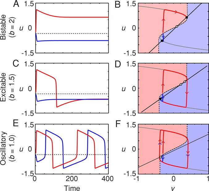
Different types of dynamics from the FHN model. (A, C, E) Time course; (B, D, F) phase plots. (A, B) Bistability. For b = 2, the system is bistable, with two stable steady states (B, filled circles) and one saddle point (B, open circle). For the value of v(t = 0) assumed here (v(t = 0) = –0.3), trajectories beginning above a threshold value of u (A, dashed line) go to the high-u stable steady state, whereas those beginning below the threshold go to the low-u stable steady state. In the phase plane, a separatrix (dashed curve) divides the starting points that approach the high-u stable steady state (pink area) from those that go to the low-u steady state. (C, D) Excitability. For b = 1.5, there is a single stable steady state plus a saddle point and an unstable steady state. Trajectories beginning above the threshold (C) or the separatrix (D) yield a pulse of u and circle the unstable steady state before settling down to a low steady-state value of u. Those beginning below the threshold do not yield a pulse of high u. (E, F) Oscillations. For b = 1.0, the single steady state is unstable. From all initial conditions (except starting right on the unstable steady state), the trajectories approach the same stable limit cycle, although from above the threshold, they go first to the upper limb of the u-nullcline, and below the threshold, they go first to the lower limb. A, C, and E are time courses; B, D, and F are phase plots. In each case, a = 0.1, ε = 0.01, v(t = 0) = −0.3, and u(t = 0) = −0.25 (red trajectories) or −0.35 (blue trajectories).