Figure 6.

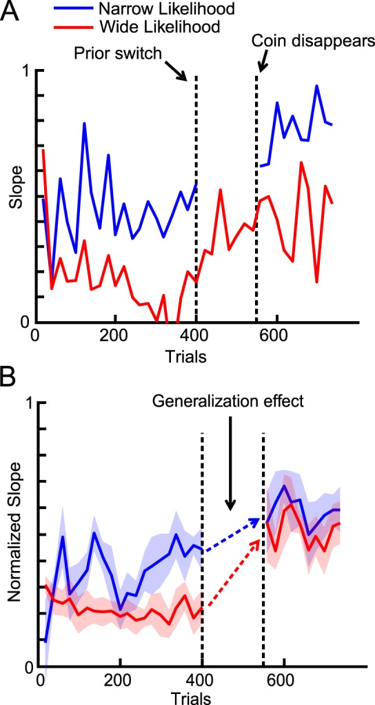
Generalization of likelihood learning (Experiment 2). (A) Data for a representative subject. Blue and red lines correspond to the narrow and wide likelihood conditions, respectively. The slope was calculated by dividing the trials into 10-trial bins and then categorizing the trials in each bin based on condition. We then calculated the slope for each condition. For this subject, the wide likelihood was used to learn the new prior. The predicted slope values from the simple Bayesian model were 0.1 (red) and 0.5 (blue) before the switch and 0.5 (red) and 0.9 (blue) after the switch. (B) Normalized slope for the likelihood that was not used during new prior learning (e.g., the blue line for the subject in [A]) averaged across all subjects. The slope was normalized in the sense that, for the subjects whose initial prior was wider, the obtained slope value was subtracted from 1 to flip the results vertically and compare them directly across different initial prior conditions. Clearly, training with one likelihood condition in the new prior learning phase carried over to the other likelihood condition (dashed arrows).