

Abstract
Type II diabetes is a growing health problem in the United States. Understanding geographic variation in diabetes prevalence will inform where resources for management and prevention should be allocated. Investigations of the correlates of diabetes prevalence have largely ignored how spatial nonstationarity might play a role in the macro-level distribution of diabetes. This paper introduces the reader to the concept of spatial nonstationarity—variance in statistical relationships as a function of geographical location. Since spatial nonstationarity means different predictors can have varying effects on model outcomes, we make use of a geographically weighed regression to calculate correlates of diabetes as a function of geographic location. By doing so, we demonstrate an exploratory example in which the diabetes-poverty macro-level statistical relationship varies as a function of location. In particular, we provide evidence that when predicting macro-level diabetes prevalence, poverty is not always positively associated with diabetes
Keywords: Diabetes, Spatial Nonstationarity, GWR, Spatial Demography, GIS, Poverty
Introduction
Type II diabetes is a growing health problem in the United States (U.S.). In 2011 diabetes affected 25.8 million Americans, and an estimated 79 million Americans had pre-diabetes (CDC, 2011). The cost of diagnosed diabetes in the U.S. was estimated at $174 billion in 2007 (CDC, 2011). Because the burden of diabetes falls disproportionately on less advantaged individuals (Kumanyika et al., 1999), poverty is one of the most important risk factors for diabetes (Levin 2011).
Micro-level (i.e. individual-level) research has consistently found positive associations between diabetes and poverty. Poverty and diabetes may be related because economic disadvantage may limit people to poorer diets and more sedentary lifestyles. For example, lower socioeconomic status is associated with prevalent diabetes among those aged 40-69 years in the United Kingdom (Connolly et al., 2000). Experiencing poverty at an early stage in life influences the likelihood of experiencing diabetes later in life (Ebrahim et al., 2004; Maty et al., 2008; Raphael, 2011). Mortality from diabetes has also been shown to be associated with family income below the poverty level (Saydah & Lochner, 2010).
Macro-level (i.e. context-level) investigations have also found a positive association between diabetes and poverty. A study using census tracts in Nashville, Tennessee, U.S.A. found diabetes to cluster in areas with high poverty (Schlundt et al., 2006). A study in Winnipeg, Manitoba, Canada, also found an association between low socioeconomic status areas and prevalence of diabetes using scan generated cluster areas (Green et al., 2003), a method that aggregates the unique combinations of small-area geographies with a high probability of clustering. Consistent with these results, rates of diabetes were higher in areas with higher economic deprivation in London, Ontario, Canada (Tompkins 2010). More recently, a study of Medicaid recipient adults in South Carolina, found that living in a persistent (≥20% of population in-poverty for each decennial years from 1970 to 2000) poverty county was positively associated with diabetes prevalence (Stewart et al., 2011). Higher area economic deprivation was also associated with higher rates of treated diabetes in French cantons (Bocquier et al., 2011).
No national studies have accounted for geographical variability in the relationship between poverty concentration and diabetes prevalence. To our knowledge, we provide this first geographically weighted analysis on the diabetes-poverty relationship over the contiguous U.S.
We introduce the reader to the concept of spatial nonstationarity. We first show how a classical ordinary least squares (OLS) regression captures the “global” and positive relationship between diabetes and poverty—where an increase in the concentration of poverty is accompanied by an increase in the prevalence of diabetes. We then make use of an exploratory geographically weighted regression (GWR) to specify a “local” model. Using this model we show that in a few instances, the diabetes-poverty statistical macro-level relationship is not positively related. Our findings reveal an example where the diabetes-poverty macro-level relationship varies by geographical space and deviates from the classical relationship—where in some areas, an increase in the concentration of poverty is accompanied by a decrease in the prevalence of diabetes.
Geographical space
Before we discuss spatial nonstationarity, we briefly introduce the “social construction of space” as a theoretical motivation of a geographically aware research agenda. In the eloquent words of Henri Lefebvre: “social space is constituted neither by a collection of things or an aggregate of (sensory) data, nor by a void packed like a parcel with various contents, and that it is irreducible to a ‘form’ imposed upon phenomena, upon things, upon physical materiality” (Lefebvre 1991:27). The interaction between individuals with each other and their physical environment produces space.
Critical spatial thinking, at its roots, arose “from the belief that we are just as much spatial as temporal beings” (Soja 2010:16 italics by original author). Said differently, physical- and social-space are both important factors within our species because we are temporal beings (see Heidegger 1962; Massey 1992). By temporal, we mean that we are most influenced by what is most immediate in space—what happens near us matters more than non-proximal events. As a consequence, we are irreversibly contemporary and unavoidably temporary (Soja 2010:15), biasing us towards the most immediate—making what happens in proximal habitats more important than events in distant spaces. The main theoretical premise in our paper is that humans' spatiality and temporality are essential and equally powerful in explaining human behavior—that they are “interwoven in a mutually formative relation” (Soja 2010:16). Consequently, the core argument in our approach is that everything that social “is simultaneously and inherently spatial, just as everything spatial, at least with regard to the human world, is simultaneously and inherently socialized” (Soja 2010:5-6).
Social structures underlying historical processes are related to current diabetes prevalence through the culmination of the existing social and physical environments. Most investigations of events do not account for to how these events unfold around geographical space. These studies fail to acknowledge if and how the distribution of events over geographical space matters. Consequently, statistical variations by geography in most research have “been treated as a kind of fixed background, a physically formed environment that, to be sure, has some influence on our lives but remains external to the social world” (Soja 2010:2). Such a theoretical approach excludes an exploration of how “geographical space” interacts with human behavior. Our study illuminates how the diabetes-poverty macro-level relationship unfolds over geographical space.
Spatial nonstationarity
Geographic spatial autocorrelation is a form of spatial dependence often exhibited in geographically referenced data. Geographic spatial autocorrelation differs from other forms of spatial dependence in that the autocorrelation arrives from the combination of the polygon's attribute and their geographical location. In 1954 statistician Peter Whittle was the first to discuss the idea of a “stationary process” in observing that new estimation techniques were necessary to model nonstationary processes—events that shifted as a function of space (Whittle 1954).
Spatial autocorrelation was formally introduced during the 1950s (e.g., Geary 1954, Moran 1950) and was mathematically defined a few years later (see Cliff 1975, Cliff and Ord 1969, 1973, 1981). Shortly thereafter, spatial autocorrelation entered the computing world (e.g., Anselin, 1980). Modeling geographic dependence has been at the forefront of sociological thought for many generations and continues to date as the discipline of spatial epidemiology evolves (Carpenter 2011).
If spatial homogeneity is present, we assume “that all members of the population have the same chance of affecting and being affected by each other” (Strang and Tuma 1993:615)—regardless of their geographical location. We expect spatial homogeneity to be rare and thus deduce, a priori, that most social phenomena are not geographically stationary In the words of Waldo Tobler (1970): “Everything is related to everything else, but near things are more related than distant things.”
Investigations on spatial nonstationarity “focus on the almost ubiquitous phenomenon that two measurements taken from geographically close locations are often more similar than measurements from more widely separated locations” (Beale et. al. 2010:247). For this reason, “spatial autocorrelation has been developed to deal with the tendency toward interdependence among spatial data” (Namboodiri 1991:221). Investigating diabetes prevalence requires we expand our understanding of how macro-level social phenomenon vary as a function of geographical distance. Our theoretical view is that the assessment of spatial nonstationarity is necessary because it can help us explicitly investigate how space plays a role in the prevalence of diabetes. In this paper we ask: Does the diabetes-poverty macro-level relationship vary by geographical location?
We believe inter-county spatial dependence is present because what happens in one county affects neighboring counties as a function of distance and that micro-level diabetes prevalence is influenced by these macro-level diffusion processes. For example, at the micro-level, economics and culture (e.g., income and exercise habits) may be playing a role in diabetes prevalence. While at the macro-level, affordable healthy food availability and physical environments that promote physical activity provide the context in which individual-level behavior can be expressed. Socioeconomic structures (like availability of good paying jobs) influence all these micro- and macro-level factors. Consequently, the contexts in which micro-level events unfold provide the material potential for an individual's behavior, and the attributes of said environments are themselves influenced by social diffusion processes (for an example on diffusion processes please see Casterline, 2001).
We first hypothesized (H1) that the macro-level relationship between percent in-poverty and diabetes prevalence is positively related in a “global” model. Next we hypothesized (H2) that the diabetes-poverty macro-level relationship will be spatially nonstationary in a “local” model. That is, after accounting for geographical location, we expect the diabetes-poverty association to fluctuate as a function of geographical location.
Data
Our data come from two secondary data sources. The Centers for Disease Control (CDC) produced 2007 county-level estimates of self-reported diabetes prevalence from the 2005-2007 Behavioral Risk Factor Surveillance Systems (BRFSS), which sampled from homes with landline telephones (CDC 2008). Social and demographic measures in the analysis come from the American Community Survey (ACS) 2005-2009 file (ACS 2011), an ongoing yearly survey that produces a randomly selected nationally-representative sample (U.S. Census Bureau, 2011).
Our independent variable of interest in both empirical models is percent of people within the county who are living below the federal poverty threshold. Poverty in the ACS is calculated using standards specified by the Office of Management and Budget based on monetary income before taxes.(U. S. Census Bureau 4). Thresholds vary by family size and composition and are annually updated for inflation using the Consumer Price Index (CPI-U). If a family's total income is less than the family's poverty threshold, then both the individual and the family are considered to be in poverty.
County shapefiles
We linked county-level measures using a geocode system that assigns a numeric or alphanumeric code to each county. We used Topological Integrated Geographic Encoding Referencing (TIGER) Shapefiles from the Census to conduct all mapping and spatial analyses. A shapefile is a geospatial vector data format used in geographic information system (GIS) related software. Shapefiles provide open specification for data interoperability by describing geometries by using points, polylines, and polygons. Full details on “.shp” files are available elsewhere (ESRI 2011). A broader explanation of U.S. Census Bureau TIGER/Line Shapefiles is also available elsewhere (U.S. Census Bureau 2007).
Although figures presented in this paper have been altered (exported from ArcMap as GIF/PDF and extracted for display in publication), the GWR analysis was conducted using shapefiles project on a U.S. contiguous Albers equal area conic USGS, using the GCS NA 1983 coordinate system with the 1983 datum and the Prime Meridian. All analyses and mapping were conducted using ArcGIS® [software by ESRI. ArcGIS® and ArcMap™ are the intellectual property of ESRI and are used herein under license (Copyright © ESRI, all rights reserved) for more information about ESRI® software, please visit www.esri.com] (For a discussion on the use of spatial statistics in ArcGIS please see Scott and Janika 2010).
Ordinary least squares regression
We first execute an OLS multivariate regression (Aiken & West, 1991) to show the linear association between diabetes prevalence and percent in-poverty in the county. The goal of this “global model” is to verify the positive association found in previous studies. Our OLS model uses percent with diabetes in the county as the dependent variable and percent in-poverty in the county as the independent variable. We control for percent of people within county who are Latinos, non-Latino-Blacks, and the percent of the county population who are immigrants as an exploratory control (Oza-Frank et al., 2011).
Geographic Weighted Regression
GWR is a modeling technique used to explore spatial non-stationarity (Brunsdon, Fotheringham, and Charlton 1996). The “main characteristic of GWR is that it allows regression coefficients to vary across space, and so the values of the parameters can vary between locations” (Mateu 2010:453). GWR is necessary when “a single global model cannot explain the relationship between some sets of variables” (Brunsdon, Fotheringham, and Charlton 1996:281). GWR allows us to explore “spatial nonstationarity by calibrating a multiple regression model which allows different relationships to exist at different” geographical locations (Leung, Mei, Zhang 2000:9). Our GWR model explores the macro-level spatial nonstationarity of the diabetes-poverty statistical relationship.
Geographers have used multilevel modeling to account for spatial variations (e.g., Jones 1991). Many have argued for use of the geographically weighted regression approach to account for spatial heterogeneity (e.g., Ali, Partridge, and Olfert 2007; Fotheringham, Charlton, and Brusdon 1996). GWR's reliability as a spatial predictor has been shown (Harris, Brunsdon, and Fotheringham 2011), and a discussion on the various statistical methods for exploring varying coefficient models can be found elsewhere (e.g., Fan and Zhang 2008; Fotheringham, Charlton, and Brunsdon 1997).
Traditional non-spatially conscious research, including our OLS approach, implicitly assumes that the nature of statistical-relationships under investigation is the same for all points within the entire study area. With GWR, we can explore how the diabetes-poverty relationship varies over space by using a geographical-space function. The OLS results are thus the “global model” findings while the GWR outputs are the “local” analysis results.
Our units of analysis in both the OLS and GWR models are counties. Our GWR model contains all the variables found in the OLS equation. In OLS, error terms are generally assumed to be independent, normally distributed random variables with a mean of zero and constant variance. This model in its unconstrained form is not implementable for investigating spatial processes because the number of parameters increases with the number of observations. Thus, we must make use of a technique for estimating a parameter “drift” (Leung, Mei, and Zhang 2000). Brunsdon et al. (1996; 1997) and others have suggested a GWR technique in which the parameters are estimated by a weighted least squares procedure. As mentioned earlier, the weighting system is dependent on the geographical location of the county. In effect, we use spatial weights that have an adaptive distance decay function. The typical output from a GWR model is a set of parameters that can be mapped in the geographic space to represent spatial nonstationarity. We use these GWR created-values (i.e., beta coefficients for each county) to map how percent in-poverty is associated with diabetes prevalence.
We use a GWR model developed by Brunsdon, Fotheringham, and Charlton (1996). In order to better understand our final GWR, we will start by describing a basic ordinary least square (OLS) linear regression model. If the standard regression equation in our investigation of diabetes is given by:
where Yi is the percent with diabetes at county i, β0 is a constant term (i.e., the intercept), and βk measures the relationship between the independent variable Xk and Y for the set of i counties, and εi is the error associated with county i.
The above equation “results in one parameter estimate for each variable included” (Cahill & Mulligan 2007). We can estimate local parameters instead of estimating single parameters for each variable. By estimating a parameter for each data location (i.e. county) in the contiguous U.S., the GWR equation would only alter the above equation as follows:
where βoi is the constant term for the corresponding explanatory variable at county i, and βki is the value of the parameter for the corresponding explanatory variable at point i, and where εi is i Є C = {1,2,…,n} and where C is the index set of locations of n observations (i.e., counties).
In the GWR model, a continuous surface of parameter values is estimated under the assumption that locations nearer to i will have more influence on the estimation of the parameter βi-hat for that location. In short, GWR asumes parameters are functions of the locations in which the observations are obtained (Brunsdon et al., 1996; Fotheringham, Brunsdon, and Charlton, 2002). Our final GWR equation using county polygons including all independent variables (in simple form) is:
When estimating spatial weights, the kernel function requires a bandwidth. A bandwidth determines the size of the kernel. A large bandwidth can produce parameters with little spatial variation. On the other hand, a small one can produce large local variation (i.e., exaggerated variance). There is no existing standard for selecting a bandwidth when using counties in a GWR model. Hence, we felt justified in using an adaptive kernel with a neighbor bandwidth that minimizes the Akaike Information Criterion (AIC), given as:
Where tr(S) is the trace of the hat matrix (Mennis, 2006). The advantage to the AIC method is that it takes into account the possible variance of the degrees of freedom using a different number of observations (for details, see Fotheringham, Brunsdon, and Charlton 2002). Roughly defined, a “kernel” is a weighting function used in the estimation of our GWR model. Kernel widths are necessary when using non-parametric estimation techniques like GWR. The kernel specifies the number of data points (i.e., the bandwidth) in the local county sample used to estimate the GWR parameters.
We focus on the 3109 counties in the contiguous U.S. because we believe our GWR analysis requires that all polygons be physically adjacent or in near physical proximity to at least one other polygon with data on the variables of interest. A “no data” polygon (i.e., 0 since “null data” will not allow the model to converge) is interpreted as a real value and could thus corrupt our GWR results.
Descriptive figures
In all our figures, we give U.S. state boundaries to better reference the colored PUMA polygons. From Figure 1, we can see that diabetes prevalence is most concentrated in the Southeastern part of the contiguous U.S. Low diabetes prevalence is present in the East. A few counties in Colorado have very low levels of diabetes prevalence.
Figure 1.

County-Level Diabetes Prevalence in 2007, Contiguous U.S.
Percent in-poverty is concentrated in the Southern part of the contiguous U.S (Figure 2). Areas with least amount of poverty concentrations can be found across the contiguous U.S. but are most concentrated in the North.
Figure 2.

County-Level Poverty Prevalence in 2005-2009, Contiguous U.S.
OLS findings
Percent in-poverty is positively related with percent with diabetes (coeff=11, Pr>|t| <0.0001, Table 1). Diabetes prevalence and percent in-poverty are positively and statistically significantly related. Our OLS findings, or the “global” model, support H1 because the relationship between percent in-poverty and diabetes prevalence is positively related.
Table 1. Association between Poverty Prevalence and Diabetes Prevalence at the County-Level.
| Estimate | SE | t Value | Pr > |t| | |
|---|---|---|---|---|
| Intercept | 8.22 | 0.07 | 110.09 | <.0001 |
| % In-Poverty | 11.00 | 0.48 | 23.16 | <.0001 |
| % Latino | -1.95 | 0.30 | -6.55 | <.0001 |
| % Non-Latino-Black | 5.54 | 0.21 | 26.53 | <.0001 |
| % Immigrants | -7.50 | 0.71 | -10.59 | <.0001 |
Using the outputs above, we contrast two hypothetical conditions. In one instance, the percent of poverty is 10%, with a 10% Latino population, 20% non-Latino-black population, and a 5% immigrant concentration. If our general equation is: predicted diabetes prevalence = 8.22 + (11*%Poverty) + (-1.95*%Latino) + (5.54*%Non-Latino-Black) + (-7.5*%Immigrant), then the equation for the case described above would be: 8.22 + (11*0.10) + (-1.95*0.10) + (5.54*0.20) + (-7.5*0.05) predicting a ∼9.9% diabetes prevalence. In a second sample, all remains the same but the percent in poverty increases to 40% so that we have an equation: 8.22 + (11*0.40) + (-1.95*0.10) + (5.54*0.20) + (-7.5*0.05) predicting a ∼13.2% diabetes prevalence. These examples demonstrate that an increase in poverty concentration is associated with an increase in diabetes at the county level.
GWR findings
We first made use of a Local Moran's I cluster analysis in the residuals of the GWR model as a diagnostic for the collinearity in GWR residuals. We found no violations of residual independence. GWR estimates in ArcGIS produced a 78 neighbor bandwidth—this is the optimal adaptive number of neighbors. Our GWR model has an R2 of 0.81 and an adjusted-R2 of 0.76. To first assess that no extreme spatial autocorrelation is present in our GWR model, we map the “condition number” values created by the procedure. The condition number is a diagnostic that evaluates local collinearity. Condition numbers larger than 30 may produce unstable results. Figure 3 displays that our data is stable in the GWR equation across counties in the contiguous U.S.
Figure 3. GWR Model Stability by County.

Local R2 values can range from 0.0 to 1.0 and indicate the fit of the model across the geographical surface under investigation. The “low values” (light-blue color in Figure 4) indicate the GWR model is predicting diabetes prevalence poorly in those places. Please note that most counties have an R2 value of 0.30 or above.
Figure 4. GWR Model Fit by County.

We find support for H2, the diabetes-poverty relationship is spatially nonstationary - it fluctuates from negative to positive (Figure 5). More technically, the degree to which the positive relationship varies by “strength” demonstrates an instance of how the classical “global association” even varies by geographical location. Most counties (yellow and greens in Figure 6) have a positive association as stipulated in H1. Out of the 3,109 counties in the contiguous U.S., 2,863 counties had positive associations between percent in-poverty and diabetes prevalence—these again lend support to the global model and H1. Although this is the majority (92%), there were 246 (8%) counties where the relationship was negative. The fluctuation in the macro-level relationship between percent in-poverty and diabetes prevalence signals that there is spatial nonstationarity in their relationship and thus supports H2 Poverty and diabetes are not always positively correlated. When geographic location is taken into account, there are a few instances where the macro-level relationship is negative (more poverty is accompanied by lower levels of diabetes prevalence).
Figure 5. GWR Associations between Poverty Prevalence and Diabetes Prevalence at the County-Level.
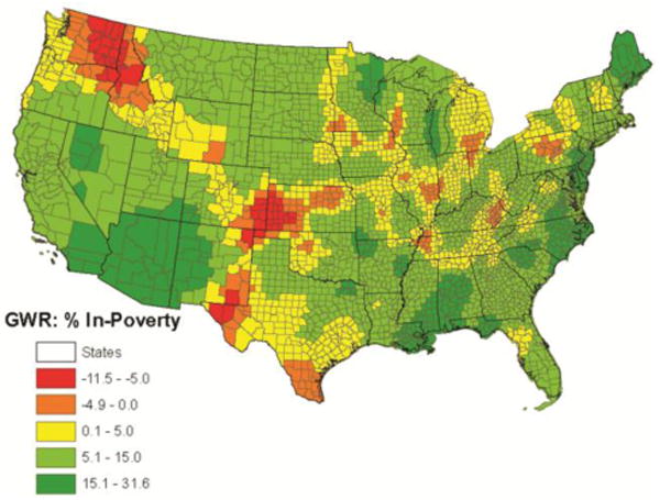
Please note that the diabetes-poverty GWR coefficient varies from -11.5 to 31.6 - this variation signals that the diabetes-poverty macro-level association is spatially nonstationary. The orange and red counties in Figure 5 indicate areas where an increase in the percent in-poverty predicts lower diabetes prevalence (GWR in-poverty coefficient ranges from -11.5 to -0.01). The shift from green counties to yellow-reds captures the spatially nonstationary relationship between poverty and diabetes. We chose not to display the associated t-values for the percent in-poverty GWR coefficient (Fotheringham et al., 1998; Huang and Leung, 2002; Lee, 2004) because of theoretical difficulties with interpreting “significance level” in GWR models where the polygon measure is an estimate instead of an “absolute and true” count (For more details on issues with mapping GWR results please see Mennis, 2006).
Discussion
Diabetes is a growing challenge in the U.S. Poverty has been a robust correlate of diabetes prevalence. Increasing our understanding of this relationship requires us to be informed of where macro-level mechanisms vary from traditional findings. We find that the macro-level diabetes-poverty relationship varies by geographical location. Results support our first formal question (H1), that at the macro-level (i.e., county-level) percent in-poverty and diabetes prevalence are positively and significantly related - as poverty levels increase so does the prevalence of diabetes. Results also support our second formal question (H2) - we find the diabetes-poverty association fluctuates from negative to positive as a function of geographical location. In short, after accounting for location, we find the diabetes-poverty macro-level association fluctuates as a function of geography. A next step in this line of research is to understand causal mechanisms in this spatially nonstationary relationship.
Our findings are limited by theoretical, modeling, and data considerations. One challenge concerns how inferences about statistical relationships drawn from areal data must be understood. Robinson long ago warned us about the aggregation problem (1950) and clearly explained that inferring individual level relationships from macro-level correlations is inappropriate. Our study uses counties as the units of analysis and its results are thus meant to be understood only as a macro-level phenomenon. Defining an appropriate measure of environment poses another limitation. Using smaller geographic units could eventually lead to “reduction ad absurdum” (Duncan, Cuzzort, and Duncan 1961:35). Earlier on the issue of scale, others concluded that in geographical investigations, “every change in scale will bring about the statement of a new problem, and there is no basis for presuming that associations existing at one scale will also exist at another” (McCarty, Hook, and Knos 1956:16). We have selected county geospatial units (i.e., polygons - irregular two-dimensional shapes made up of straight sides) based on data availability rather than theoretical grounds. For these reasons our analysis should be seen as exploratory.
Our GWR model also presents some limitations because it is an exploratory technique, as statistical inferences from spatial modeling are still being debated (Anselin 2005; Ripley 1981; 1988). Specialists in the field have pointed out that in “order to carry out statistical inference, a notion of a super population or spatial random process is required” where we would have to assume the existence “of a stochastic process that may generate many possible spatial patterns” and where the main objective of the analysis would be “to characterize the spatial process by means of the observed spatial pattern” (Anselin 2005:255). We do not have a reference super population, and we make use of “estimates” that have standard errors. As specified, our GWR model has no way of accounting for the fact that we are using sample data - and thus the different confidence intervals in the estimates as it explores their relationship as a function of geographical location.
Beyond these statistical matters, there are some limitations present in our data. For example, diabetes status is self-reported and only recorded as such if a person has been formally diagnosed by a health care professional. Our BRFSS sample data was created from a “landline-phones” universe and will therefore exclude certain households without such telephones. Despite these limitations, we believe “GWR analysis serves as an exploratory geographic analysis tool to detect local anomalies” (Qiu and Wu 2010:80 Huang and Leung, 2002; Lee, 2004). Our GWR analysis demonstrates the existence of geographic spatial nonstationarity. Most, but not all, areas with a negative relationship between poverty and diabetes are rural. Future studies should examine how the variation in the availability of resources such as grocery stores, convenience stores, fast food outlets, and full-service restaurants in rural areas (Ahern 2011—see citation below) influences this relationship. Additional research should investigate factors related to this negative relationship specific to the urban areas of South and Western Texas and Detroit.
In the early 20th century, Park stated that “is because social relations are so frequently and so inevitably correlated with spatial relations…that statistics have any significance” whatsoever for those who investigate human behavior (Park 1926:18). Humans' temporal disposition obligates social scientist to continue exploring how space affects human behavior. Mitigating the U.S. diabetes epidemic necessitates addressing how the spatially nonstationary macro-level relationship between diabetes and poverty can inform micro-level processes.
References
- Aiken LS, West SG. Multiple Regression: Testing and Interpreting Interactions. Sage; Thousand Oaks, California: 1991. [Google Scholar]
- Ali K, Partridge MD, Olfert MR. Can Geographically Weighted Regressions Improve Regional Analysis and Policy Making? International Regional Science Review. 2007;30:300–329. [Google Scholar]
- Anselin L. Under the Hood. Issues in the Specification and Interpretation of Spatial Regression Models. Agricultural Economics. 2005;27:247–267. [Google Scholar]
- Anselin L. Estimation Methods for Spatial Autoregressive Structures: A Study in Spatial Econometrics, Regional Science Dissertation and Monograph Series #8. Program in Urban and Regional Studies Publications; Ithaca, N.Y: 1980. [Google Scholar]
- Brunsdon C, Fotheringham AS, Charlton ME. Geographically Weighted Regression: A Method for Exploring Spatial Nonstationarity. Geographical Analysis. 1996;28:281–298. [Google Scholar]
- Cahill M, Mulligan G. Using Geographically Weighted Regression to Explore Local Crime Patterns. Social Science Computer Review. 2007;25:174–193. [Google Scholar]
- Carpenter TE. The spatial epidemiologic (r)evolution: A look back in time and forward to the future. Spatial and Spatio-temporal Epidemiology. 2011;2:119–124. doi: 10.1016/j.sste.2011.07.002. [DOI] [PubMed] [Google Scholar]
- Casterline JB. Diffusion Processes and Fertility Transition: Introduction. In: Casterline JB, editor. Diffusion Processes and Fertility Transition. National Academy Press; Washington D.C.: 2001. pp. 1–38. [PubMed] [Google Scholar]
- CDC. 2008, County level estimates of diagnosed diabetes---U S maps. Atlanta, GA: CDC; 2008. Available at http://apps.nccd.cdc.gov/ddt_strs2/nationaldiabetesprevalenceestimates.aspx. [Google Scholar]
- CDC 2011, Centers for Disease Control and Prevention. National Diabetes Fact Sheet: national estimates and general information on diabetes and prediabetes in the United States, 2011. Atlanta, GA: U.S. Department of Health and Human Services, Centers for Disease Control and Prevention; 2011. [Google Scholar]
- Cliff AD. Elements of Spatial Structure: A Quantitative Approach. Cambridge University Press; London: 1975. [Google Scholar]
- Cliff AD, Ord JK. The Problem of Spatial Autocorrelation. In: Scott AJ, editor. London Papers in Regional Science. Pion; London: 1969. pp. 25–55. [Google Scholar]
- Cliff AD, Ord JK. Spatial Autocorrelation. Pion; London: 1973. [Google Scholar]
- Cliff AD, Ord JK. Spatial Processes: Models and Applications. Pion; London: 1981. [Google Scholar]
- Connolly V, Unwin N, Sherriff P, Biolous R, Kelly W. Diabetes prevalence and socioeconomic status: a population based study showing increased prevalence of type 2 diabetes mellitus in deprived areas. Journal of Epidemiology & Community Health. 2000;54:173–177. doi: 10.1136/jech.54.3.173. [DOI] [PMC free article] [PubMed] [Google Scholar]
- Duncan OD, Cuzzort RP, Duncan B. Statistical Geography: Problems in Analyzing Areal Data, U S. The Free Press of Glencoe; Illinois, Glencoe: 1961. [Google Scholar]
- Ebrahim S, Montaner D, Lawlor DA. Clustering of Risk Factors and Social Class in Childhood and Adulthood in British Women's Heart and Health Study: Cross Sectional Analysis. BMJ. 2004;328:861–866. doi: 10.1136/bmj.38034.702836.55. [DOI] [PMC free article] [PubMed] [Google Scholar]
- ESRI. ArcGIS Desktop: Release 10. Redlands, CA: Environmental Systems Research Institute; 2011. [Google Scholar]
- Fotheringham AS, Brundson C, Charlton ME. Geographically Weighted Regression: The Analysis of Spatially Varying Relationships. John Wiley; West Sussex, UK: 2002. [Google Scholar]
- Fotheringham AS, Charlton ME, Brunsdon C. The Geography of Parameter Space: An Investigation into Spatial Non-Stationarity. International Journal of Geographic Information Systems. 1996;10:605–627. [Google Scholar]
- Geary RC. The Contiguity Ratio and Statistical Mapping. The Incorporated Statistician. 1954;5:115–145. [Google Scholar]
- Harris P, Brunsdon C, Fotheringham AS. Links, Comparisons and Extension of the Geographically Weighted Regression Model when used as a Spatial Predictor. Stochastic environmental Research and Risk assessment. 2011;25:123–138. [Google Scholar]
- Heidegger M. In: Being and Time. Macquarrie John, Robinson Edward., translators. Harper & Row Inc; New York: 1962. [Google Scholar]
- Huang Y, Leung Y. Analyzing regional industrialization in Jiangsu province using geographically weighted regression. Journal of Geographical Systems. 2002;4:233–249. [Google Scholar]
- Jones K. Specifying and Estimating Multi-Level Models for Geographical Research. Transactions of the Institute of British Geographers. 1991;16:148–160. [Google Scholar]
- Kumanyika SK. Understanding Ethnic Differences in Energy Balance: Can we get there from Here? American Journal of Clinical Nutrion. 1999;70:1–2. doi: 10.1093/ajcn/70.1.1. [DOI] [PubMed] [Google Scholar]
- Lee SI. Spatial data analysis for the US regional income convergence, 1969–1999: a critical appraisal of b-convergence. Journal of the Korean Geographical Society. 2004;39:212–228. [Google Scholar]
- Lefebvre H. In: The Production of Space. Nicholson-Smith Donald., translator. Blackwell; UK: 1991. [Google Scholar]
- Leung Y, Mei C, Zhang W. Statistical Test for Spatial Nonstationarity Based on the Geographically Weighted Regression Model. Environment and Planning. 2000;32:9–32. [Google Scholar]
- Mateu J. Comments On: A Gernal Science-Based Framework for Dynamical Spatio-Temporal Model. Test. 2010;19:452–455. [Google Scholar]
- Massey DB. Politics and Space/Time. New Left Review. 1992;1:65–84. [Google Scholar]
- Maty SC, Lynch JW, Raghunathan TE, Kaplan GA. Childhood Socioeconomic Position, Gender Adult Body Mass Index, and Incidence of Type 2 Diabetes Mellitus over 34 Years in the Alameda County Study. American Journal of Public Health. 2008;98:1486–1494. doi: 10.2105/AJPH.2007.123653. [DOI] [PMC free article] [PubMed] [Google Scholar]
- McCarty HH, Hook JC, Knos DS. The Measurement of Association in Industrial Geography. Department of Geography, State University of Iowa; Iowa City: 1956. [Google Scholar]
- Moran P, Pierce A. Notes on Continuous Stochastic Phenomena. Biometrika. 1950;37:17–23. [PubMed] [Google Scholar]
- Namboodiri K. Demographic Analysis: A Stochastic Approach. Academic Press Inc; New York: 1991. [Google Scholar]
- Oza-Frank R, Stephenson R, Venkat Narayan KM. Diabetes Prevalence by Length of Residence Among US Immigrants. Journal of Immigrant Minority Health. 2011;13:1–8. doi: 10.1007/s10903-009-9283-2. [DOI] [PubMed] [Google Scholar]
- Park RE. The Urban Community as a Spatial Pattern and a Moral Order. In: Burgess EW, editor. The Urban Community. University of Chicago Press; Chicago: 1926. [Google Scholar]
- Raphael D. Poverty in childhood and adverse health outcomes in adulthood. Social Science & Medicine. 2011;69:22–26. doi: 10.1016/j.maturitas.2011.02.011. [DOI] [PubMed] [Google Scholar]
- Ripley BD. Spatial Statistics. John Wiley and Sons, Inc; New Jersey: 1981. [Google Scholar]
- Ripley BD. Statistical Inference for Spatial Processes. Cambridge University Press; New York: 1988. [Google Scholar]
- Saydah S, Lochner K. Socioeconomic Status and Risk of Diabetes-Related Mortality in the U.S. Public Health Reports. 2010;125:377–388. doi: 10.1177/003335491012500306. [DOI] [PMC free article] [PubMed] [Google Scholar]
- Scott LM, Janikas MV. Spatial Statistics in ArcGIS. In: Fischer MM, Getis A, editors. Handbook of Applied Spatial Analysis: Software Tools, Methods and Applications. Springer-Verlag; Berlin: 2010. [Google Scholar]
- Soja EW. Seeking Spatial Justice. University of Minnesota Press; Minneapolis: 2010. [Google Scholar]
- Stewart JE, Battersby SE, Lopez-De Fede A, Remington KC, Hardin JW, Mayfield-Smith K. Diabetes and the socioeconomic and built environment: geovisualization of disease prevalence and potential contextual associations using ring maps. International Journal of Health Geographics. 2011;10 doi: 10.1186/1476-072X-10-18. [DOI] [PMC free article] [PubMed] [Google Scholar]
- Tobler W. A Computer Movie Simulating Urban Growth in the Detroit Region. Economic Geography. 1970;46:234–240. [Google Scholar]
- U.S. Census Bureau. Technical Documentation prepared by the US Census Bureau. Washington, DC: 2007. 2007 TIGER/Line Shapefiles. [Google Scholar]
- U.S. Census Bureau. Technical Documentation prepared by the US Census Bureau. Washington, DC: 2011. American Community Survey, Public Use Microdata Sample 2005-2009. [Google Scholar]
- Whittle P. On Stationary Processes in the Plane. Biometrika. 1954;41:434–449. [Google Scholar]