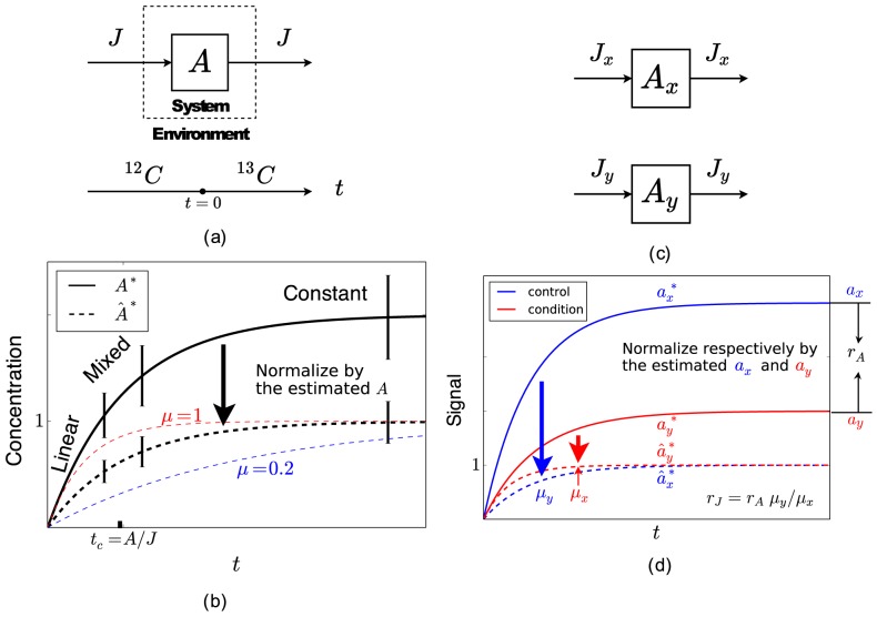
Figure 1. Understanding KFP and rKFP.
(a) A schematic diagram of KFP applied to a toy metabolic network. At  , the system is switched from a
  C-labeled environment to
  C-labeled one, and
  is measured at a few time points thereafter. (b) For a given trajectory of
  (the black solid curve), the three time regimes (linear, mixed and constant) are marked and three measurements are made (two in the mixed regime and one in the constant). Normalizing it gives
  between 0 and 1 (the black dashed curve), parameterized by a single parameter
  , which can be estimated by comparing the normalized measurements to
  's of different
  's (the red and blue dashed curves). (c) A schematic diagram of rKFP applied to the same network in (a). Relative quantitation is performed on
  in two conditions (with subscripts
  and
and  respectively) with the goal of estimating
  . (d) The ratio in
  between
  and
and  is
is  (Eq. 6), and since
  's and
  are identifiable from relative quantitation, so is
  .
.

