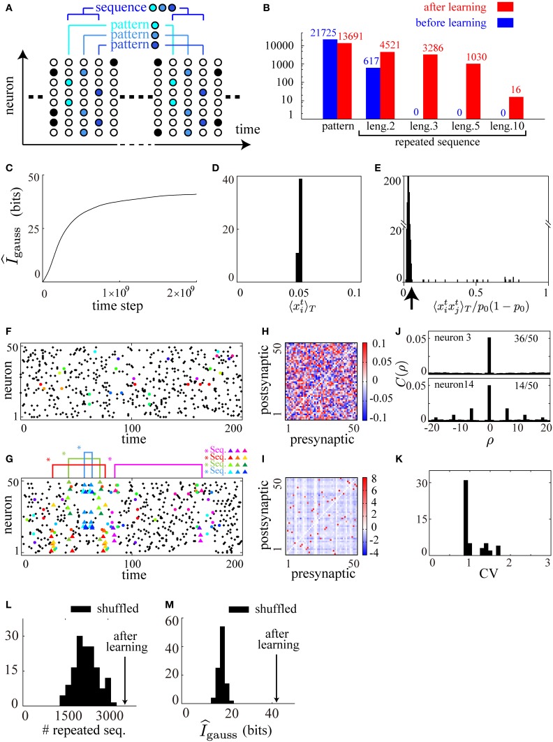
Figure 2.
Cell-assembly-like repeated sequences of firing patterns are reproduced by applying the learning rule to a spontaneously firing recurrent neural network. (A) A schematic illustration of the definition of firing patterns and of sequences of firing patterns. Each color represents a unique firing pattern xt ∈ {0, 1}N. A repeated sequence of firing patterns of length 3 {xt, xt − 1, xt − 2} ∈ {0, 1}3N is also illustrated. (B) Comparison of the numbers of firing patterns and repeated sequences (repeated more than twice) of length 2, 3, 5, and 10 before and after learning, counted for a particular 50000 time steps in the simulation. (C) The approximate measure of the mutual information gauss is calculated during the course of learning. (D) A histogram of mean firing rates of the neurons in the network after learning. (E) A histogram of pairwise correlations between all the pairs of neurons in the network after learning. (F,G) Typical raster plots before (F) and after (G) learning in which repeated sequences are represented as triangles of different colors, repeated patterns as filled circles of different colors, and other spikes as black dots, according to the definition illustrated in (A). (H,I) Connection weight matrices of the network before (H) and after (I) learning in which rows correspond to connections to single postsynaptic neurons while columns correspond to connections from single presynaptic neurons. (J) Typical two examples from the autocorrelograms calculated from the activity of each neuron in the network after learning. Thirty-six of the neurons show no autocorrelation as seen in the upper figure, while fourteen show damped periodicity as seen in the lower figure. (K) A histogram of CV values calculated from the activity of each neuron in the network after learning. (L,M) Comparison of gauss (L) and the numbers of sequences of length 3 (counted for a particular 50000 time steps) (M) of the network after learning (arrows) with those of one hundred shuffled networks (histograms). The following parameters have been used in this simulation: ϵ = 0.006, cη = 1.5, cκ = 1.0, cζ = 3.0, p0 = 0.05, pmax = 0.95, N = 50, τ = 15, T = 50000.

