Signal to noise ratio of energy selective x-ray photon counting systems with pileup

Abstract

Purpose:

To derive fundamental limits on the effect of pulse pileup and quantum noise in photon counting detectors on the signal to noise ratio (SNR) and noise variance of energy selective x-ray imaging systems.

Methods:

An idealized model of the response of counting detectors to pulse pileup is used. The model assumes a nonparalyzable response and delta function pulse shape. The model is used to derive analytical formulas for the noise and energy spectrum of the recorded photons with pulse pileup. These formulas are first verified with a Monte Carlo simulation. They are then used with a method introduced in a previous paper [R. E. Alvarez, “Near optimal energy selective x-ray imaging system performance with simple detectors,” Med. Phys. 37, 822–841 (2010)] to compare the signal to noise ratio with pileup to the ideal SNR with perfect energy resolution. Detectors studied include photon counting detectors with pulse height analysis (PHA), detectors that simultaneously measure the number of photons and the integrated energy (NQ detector), and conventional energy integrating and photon counting detectors. The increase in the A-vector variance with dead time is also computed and compared to the Monte Carlo results. A formula for the covariance of the NQ detector is developed. The validity of the constant covariance approximation to the Cramèr–Rao lower bound (CRLB) for larger counts is tested.

Results:

The SNR becomes smaller than the conventional energy integrating detector (Q) SNR for 0.52, 0.65, and 0.78 expected number photons per dead time for counting (N), two, and four bin PHA detectors, respectively. The NQ detector SNR is always larger than the N and Q SNR but only marginally so for larger dead times. Its noise variance increases by a factor of approximately 3 and 5 for the A₁ and A₂ components as the dead time parameter increases from 0 to 0.8 photons per dead time. With four bin PHA data, the increase in variance is approximately 2 and 4 times. The constant covariance approximation to the CRLB is valid for larger counts such as those used in medical imaging.

Conclusions:

The SNR decreases rapidly as dead time increases. This decrease places stringent limits on allowable dead times with the high count rates required for medical imaging systems. The probability distribution of the idealized data with pileup is shown to be accurately described as a multivariate normal for expected counts greater than those typically utilized in medical imaging systems. The constant covariance approximation to the CRLB is also shown to be valid in this case. A new formula for the covariance of the NQ detector with pileup is derived and validated.

1. INTRODUCTION

One of the most important advantages^1,2 of photon counting detectors for medical x-ray systems is their ability to provide energy spectrum information with pulse height analysis (PHA).³ However, the adoption of these detectors has been limited because the current state-of-the-art response time, or dead time, is large compared with the interphoton times of the high count rates required for medical applications. The dead time leads to pulse pileup³ that distorts the count signals and the recorded energy. These distortions affect the performance of energy selective systems and the purpose of this paper is to derive fundamental limits on the effect of pileup on the signal to noise ratio (SNR) and noise variance of these systems.

Photon counting detectors have a number of imperfections that affect their use in medical imaging systems.^1,2,4–9 This paper focuses on the fundamental limitations of finite response time and quantum noise. These are both fundamental limitations that will be present in all detectors. The universal presence of quantum noise is well known but, due to the random interaction times of photons with matter,¹⁰ there will always be a nonzero probability that two or more interactions may occur during the detector response time no matter how small. These multiple interactions affect the signal and the noise and we need methods to quantify their effects and to compare the performance of different types of detectors.

In order to focus on the effects of finite response time, an idealized model of photon counting detectors will be used. The model assumes a nonparalyzable response and delta function pulse shape. With the nonparalyzable model, the dead time is fixed and unaffected by the arrival of other photons during the lock up period. The delta function pulse shape implies that the recorded energy is the sum of the energies of the photons that arrive during the dead time regardless of how close the arrival time of additional photons to the end of the period.

The idealized model is used to derive analytical formulas for the noise and energy spectrum of the recorded photons with pulse pileup. These formulas are first verified with a Monte Carlo simulation that compares the covariance of A-vector noise to the Cramèr–Rao lower bound (CRLB). They are then used with a method introduced in a previous paper¹¹ to compare the signal to noise ratio of systems using detectors with pileup to the ideal Tapiovaara–Wagner¹² SNR with perfect energy resolution. The method is applied to compute the SNR as a function of dead time of several types of detectors including photon counting detectors with pulse height analysis, detectors that simultaneously measure the number of photons and the integrated energy,^13,14 called NQ detectors here, and conventional energy integrating and photon counting detectors. The increase in the A-vector variance with dead time is also computed and compared to the Monte Carlo results.

Mathematical models of the statistical properties of the signals of photon counting detectors with pileup are described. A new mathematical model for the covariance of NQ signals with pileup is derived and validated with Monte Carlo simulations. Methods to compute the CRLB are discussed. It is shown that the constant covariance approximation to the CRLB introduced in a previous paper¹⁵ also provides accurate results for detectors with pulse pileup. The constant covariance model is easier to compute and leads to simpler analytical formulas.

2. METHODS

2.A. The Tapiovaara–Wagner optimal SNR with full energy spectrum information

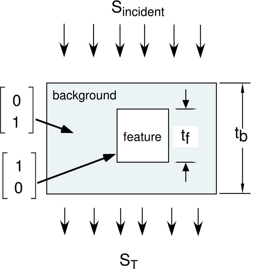
In order to compare the SNR of energy selective systems, we need to define an imaging task. The task used by Tapiovaara and Wagner¹² will also be used. The task, shown in Fig. 1, is to decide from measurements of the spectrum of the transmitted photons whether a feature is present or not. Two measurements are made, the first in the background region and the second in a region that may or may not contain the feature. The object is composed of two uniform materials, background and feature, and has a constant thickness.

FIG. 1.

Imaging task for SNR computation. The object consists of a slab of background material that may have an embedded feature. It is irradiated with an energy spectrum S_incident(E) and the transmitted photons with energy spectrum S_T(E) are measured by an energy selective detector in the background region and in the region with the feature. The task is to decide from the spectrum measurements whether the feature is present.

Tapiovaara and Wagner showed that with a quantum noise limited detector with no pulse pileup, the SNR is

$${\displaystyle {\mathrm{SNR}}^2=\frac{{\left[\int \left[S_b\left(E\right)-S_f\left(E\right)\right]D\left(E\right)w\left(E\right)\mathrm{d}E\right]}^2}{\int \left[S_b\left(E\right)+S_f\left(E\right)\right]D\left(E\right)w^2\left(E\right)\mathrm{d}E},}$$

where S_b(E) and S_f(E) are the mean spectra in the background and feature measurement regions at x-ray energy E, D(E) is the fraction of the photons detected, and w(E) is a weighting or coding function. They then showed that for an ideal detector that maximizes SNR, D(E) = 1 and

$${\displaystyle w\left(E\right)=\frac{S_b\left(E\right)-S_f\left(E\right)}{S_b\left(E\right)+S_f\left(E\right)}.}$$

With these parameters, the optimal SNR is

$${\displaystyle {\mathrm{SNR}}_{\mathrm{ideal}}^2=\int \frac{{\left[S_b\left(E\right)-S_f\left(E\right)\right]}^2}{S_b\left(E\right)+S_f\left(E\right)}\mathrm{d}E.}$$

If the feature is thin so $t_f\left[{\mu }_f\left(E\right)-{\mu }_b\left(E\right)\right]\ll 1$, then the optimal SNR is

$${\displaystyle {\mathrm{SNR}}_{\mathrm{ideal,Tapiovaara-Wagner}}^2=\frac{t_f^2}{2}\int S_b\left(E\right){\left[\delta \mu \left(E\right)\right]}^2\mathrm{d}E,}$$

where δμ(E) = μ_f(E) − μ_b(E). We can gain some insight into this expression by defining a normalized spectrum

$${\displaystyle {\hat{S}}_b\left(E\right)=\frac{S_b\left(E\right)}{\int S_b\left(E\right)\mathrm{d}E}.}$$

Then,

$${\displaystyle {\mathrm{SNR}}_{\mathrm{ideal,Tapiovaara-Wagner}}^2=\lambda \frac{t_f^2}{2}{〈{\left[\delta \mu \left(E\right)\right]}^2〉}_{S_b},}$$ (1)

where λ = ∫S_b(E)dE is the expected number of photons and

$${\displaystyle {〈{\left[\delta \mu \left(E\right)\right]}^2〉}_{S_b}=\int {\hat{S}}_b\left(E\right){\left[\delta \mu \left(E\right)\right]}^2\mathrm{d}E}$$

is the effective value of the square of the difference of the attenuation coefficients using the normalized energy spectrum as the weighting function.

2.B. Linearized model for noise analysis

Applying the Alvarez–Macovski method¹⁶ to the Tapiovaara–Wagner imaging task, the x-ray attenuation coefficient μ(r, E) at each point r in the object at photon energy E is approximated as a linear combination of basis functions

$${\displaystyle \mu (\mathbf{r},E)=a_1\left(\mathbf{r}\right)f_1\left(E\right)+a_2\left(\mathbf{r}\right)f_2\left(E\right).}$$ (2)

In this paper, two basis functions will be used, which is accurate for ordinary body materials.¹⁵ Following the method introduced in a previous paper,¹¹ we can apply the decomposition in Eq. (2) to the imaging task in Fig. 1 by letting the attenuation coefficients of the background and feature materials be the basis functions. Then, the vectors of the basis set coefficients, $\mathbf{a}={\left[a_1,a_2\right]}^T$, for the feature and background regions are

$${\displaystyle {\mathbf{a}}_{\mathbf{f}}=\left[\begin{array}{c}\hfill 1\hfill \\ \hfill 0\hfill \end{array}\right],{\mathbf{a}}_{\mathbf{b}}=\left[\begin{array}{c}\hfill 0\hfill \\ \hfill 1\hfill \end{array}\right].}$$ (3)

Column vectors are used and the symbol T denotes a transpose.

We solve for the A-vector, the vector whose components are line integrals of the basis coefficients A_j = ∫_Patha_j(r)dsj = 1, 2, by using measurements of the transmission of the object with multiple spectra. With a photon counting detector, the expected values of the measurements are

$${\displaystyle N_j=\int g_j\left(E\right)S\left(E\right)e^{-A_1{f}_1\left(E\right)-A_2{f}_2\left(E\right)}\mathrm{d}Ej=1,\hspace{0.17em}\dots ,\hspace{0.17em}J,}$$ (4)

where S(E) is the spectrum transmitted through the object and g_j(E) are the effective spectra for the measurements. For example, with ideal PHA, the g_j(E) are rectangle functions equal to 1 in each energy bin and 0 outside.

Because of the exponential relation of measurements to the A-vector in Eq. (4), taking the logarithm approximately linearizes it. Defining the logarithm of the measurements vector L with components

$${\displaystyle L_j=-log\left(\frac{N_j}{N_j\left(0\right)}\right),}$$

where N_j(0) is the measurement with no object in the beam, we can approximate the measurement for noise calculations using the linear term of the Taylor’s series about the expected value $〈\mathbf{A}〉$

$${\displaystyle \delta \mathbf{L}\left(\mathbf{A}\right)\approx \frac{\partial \mathbf{L}}{\partial \mathbf{A}}\delta \mathbf{A}+\cdots .}$$ (5)

In Eq. (5), $\delta \mathbf{L}=\mathbf{L}(〈\mathbf{A}〉+\delta \mathbf{A})-\mathbf{L}\left(〈\mathbf{A}〉\right)$ and $\delta \mathbf{A}=\mathbf{A}-〈\mathbf{A}〉$ are the deviations about the expected value.

2.C. Comparing the SNR of detectors

With the linearized model of Eq. (5) and assuming that the noise probability distribution is multivariate normal, we can apply statistical detection theory to analyze the performance in the imaging task of Fig. 1. If the feature does not have high attenuation so the covariance of the A-vector, C_A, is approximately the same in the background and feature regions, the signal to noise ratio is

$${\displaystyle {\mathrm{SNR}}^2={\left(\delta \mathbf{A}\right)}^T{\mathbf{C}}_{\mathbf{A}}^{-1}\delta \mathbf{A}.}$$ (6)

The use of the multivariate normal distribution is examined in Appendix A and the constant covariance assumption is discussed in Appendix B. The Appendices show that both of these assumptions are justified for sufficiently large expected number of photons. Since medical x-ray imaging systems for material-selective applications typically use large number of photons per measurement, the assumptions are justified for the systems to be studied here.

The optimal SNR for any detector can be computed by using the constant covariance CRLB for C_A,¹⁷

$${\displaystyle {\mathbf{C}}_{\mathbf{A}}={\left({\mathbf{M}}^{\mathbf{T}}{\mathbf{C}}_{\mathbf{L}}^{-1}\mathbf{M}\right)}^{-1},}$$ (7)

where the notation ${\left(\right)}^{-1}$ denotes the matrix inverse and M = ∂L/∂A is the gradient of the measurements as defined in Eq. (5).

In Eq. (6), δA is the difference of the A-vectors of the feature and background regions in Fig. 1

$${\displaystyle \delta \mathbf{A}={\mathbf{A}}_{\mathbf{feature}+\mathbf{background}}-{\mathbf{A}}_{\mathbf{background}}.}$$

With the parallel geometry, the A-vectors are A_{feature+background} = a_b(t_b − t_f) + a_ft_f and A_background = a_bt_b, where a_b and a_f are the basis set coefficients of the background and feature materials given in Eq. (3). The difference of the A-vector is therefore

$${\displaystyle \delta \mathbf{A}=t_f\left({\mathbf{a}}_{\mathbf{f}}-{\mathbf{a}}_{\mathbf{b}}\right)=t_f\left[\begin{array}{c}\hfill 1\hfill \\ \hfill -1\hfill \end{array}\right].}$$

By using this result in Eq. (6), we can compare the SNR derived with the basis function decomposition to the Tapiovaara–Wagner optimal SNR in Eq. (1).

2.D. Models for pulse pileup

The x-ray photon counting detectors analyzed here have two principal components: a sensor that interacts with x-ray photons and produces a signal and a readout that analyzes the signal. An example of a sensor is a high atomic number semiconductor material. X-ray photons produce free charge carriers in the material and it takes a finite time to collect them. The readout electronics also require a finite time to carry out their operations. These effects and others^2,4 result in a nonzero overall detector response time and there will be errors if photons enter the sensor during the response time of a first photon resulting in pulse pileup.

Pulse pileup is a complex phenomenon that affects both the recorded counts and photon energies.² These signals depend on the pulse waveform and, due to the differing mobilities of electrons and holes and many other factors, the waveform can be complex with a peak and long tail.^8,18 However, as has been shown by the use of silicon with its excellent material properties as a sensor,¹ as the properties of high atomic number semiconductors improve, the pulse shapes approach an ideal short time pulse. Therefore, idealized models will be emphasized here to derive fundamental limits.

Two general models have been developed to describe the effect of pulse pileup on recorded counts,³ paralyzable and nonparalyzable. The purpose of these models is to describe the signals as a function of count rate and not necessarily the actual functioning of a detector. In both models, the total response time is modeled using the dead time, τ, which is defined to be the minimum time between two photons that are recorded as separate events.³ The dead time combines the contributions of both the sensor and readout response times. In both models, the detector is assumed to start in a “live” state. When a photon is absorbed, the detector is modeled as entering a separate state where it does not count additional photons. In the paralyzable model, the arrival of photons extends the time in the noncounting state. In the nonparalyzable model, the time in the separate state is assumed to be fixed and independent of the arrival of any other photons during the dead time. Both models give similar recorded counts at low interaction rates but give different results at high rates where the probability of multiple interactions during the dead time becomes significant. The nonparalyzable model will be used in this paper. Measurements by Taguchi et al.⁸ indicate that for the detectors they studied it is more accurate at higher count rates. It also leads to simpler analytical results.¹⁹

The recorded energy with pileup will be modeled with an idealization that assumes the pulse shape is a delta function and the recorded energy is the integral of the pulses during the dead time.⁹ With this approximation, the detector dead time is modeled separately from pulse width and is not due to overlapping pulses. The model also assumes that the photon energy is converted completely and linearly into charge carriers so there are no losses due to Compton or Rayleigh scattering and all K-fluorescence radiation is reabsorbed within the sensor. All of the carriers are assumed to be collected so there is no charge trapping or charge sharing with nearby detectors. With these assumptions, the recorded energy is the sum of the energies of the photons that arrive during the dead time regardless of how close the arrival of a photon to the end of the period.

The recorded energies are sum of several random quantities including the random photon energies produced by the x-ray source, the random number of charge carriers produced by a photon of a given energy, electronic noise in the readout, and others. An energy of the order of 10 electron-volts (eV) is required to produce a charge carrier pair in common x-ray sensors⁴ and diagnostic x-ray photon energies are of the order of 10⁵ eV, so an average, $〈N_e〉$, 10⁴ charge carrier pairs are produced by each photon. Assuming the number of carriers is Poisson distributed, it can be shown that the standard deviation of the measured energy errors due to the random number of charge carriers is $〈E〉/\sqrt{〈N_e〉}$, where $〈E〉$ is the average photon energy incident on the detector. With the large number of charge carriers produced, this is much less than the standard deviation of the photon energies of a broad spectrum source such as an x-ray tube that is almost universally used in material-selective imaging.

Similarly, noise in modern electronics can be reduced so its contribution to the standard deviation of the measured energy errors is also much less than the photon energy standard deviation. The random factors can be modeled as statistically independent so the probability density function (PDF) of the recorded photon energies is the convolution of their individual PDF.²⁰ Because the variances of the other factors are much smaller, the overall PDF will be dominated by the photon energy PDF. The overall recorded energy PDF will therefore be modeled as depending only on the photon energy spectrum incident on the detector and the dead time as described in Secs. 2.G and 2.H.

2.E. Photon count statistics with pileup

A widely used model¹⁰ for the number of photons N(t) incident on the detector before time t is a Poisson counting process. With this process, the random interevent times have an exponential distribution. If t_n is the time of event n, then the probability that the next event time t_n+1 is less than t_n + δt is

$${\displaystyle \mathrm{Prob}(t_{n+1}<t_n+\delta t)=1-e^{-\rho \delta t},\delta t\ge 0,}$$ (8)

where, as defined in Sec. 2.D, ρ is the average rate of photon arrivals. For small δt, this is approximately ρδt so the probability that one or more photons arrive during the response time τ is greater than ρτ. For a nonzero τ, there is always a nonzero probability that one or more photons arrive during this time. For later use, note that²¹ the expected value of the exponentially distributed interevent times is 1/ρ and the variance is 1/ρ².

With pulse pileup, we can describe the recorded counts as a renewal process where the interevent times are not necessarily exponentially distributed as in the Poisson process. Suppose the expected value and variance of the interevent times are μ and σ and N(t) is the number of photons that have arrived by time t. The central limit theorem of renewal processes²² states that, for counting times much greater than the mean interevent time, we can standardize N(t) so that the distribution of

$${\displaystyle \frac{N\left(t\right)-t/\mu }{\sigma \sqrt{t/{\mu }^3}}\to \mathcal{N}(0,1)}$$ (9)

approaches a normal distribution with zero mean and unit variance. This theorem is reasonable since if t is much greater than the mean interevent time, N(t) depends on the sum of a large number of random interevent times.

Applying the theorem to the nonparalyzable case with dead time τ, the mean interevent time of the recorded photons increases to ${\mu }_{\mathrm{pileup}}=\left(1/\rho \right)+\tau$. Since τ is constant, the variance is unchanged ${\sigma }_{\mathrm{pileup}}^2=1/{\rho }^2$. From Eq. (9), for counting times substantially larger than 1/ρ, the mean and variance with pileup approach the following limiting values:

$${\displaystyle 〈N_{\mathrm{rec}}\left(t\right)〉\to t/{\mu }_{\mathrm{pileup}}=\frac{\lambda }{1+\eta },}$$ (10)

$${\displaystyle \text{Var}\left(N_{\mathrm{rec}}\right(t\left)\right)\to {\sigma }_{\mathrm{pileup}}^{2}t/{\mu }_{\mathrm{pileup}}^3=\frac{\lambda }{{\left(1+\eta \right)}^3},}$$ (11)

where λ = ρt is the expected number of photons incident on the detector during the measurement time and η = ρτ is the expected number during the dead time. With η greater than zero, the statistics are no longer Poisson since the expected value and the variance are different.

2.F. Statistics of NQ detectors with pileup

The NQ detector simultaneously measures the count N and the integrated energy Q of the photons. Alvarez¹¹ showed that the covariance with no pulse pileup is

$${\displaystyle {\mathbf{C}}_{\mathbf{NQ},\mathbf{no}\mathbf{pileup}}=\lambda \left[\begin{array}{cc}\hfill 1\hfill & \hfill 〈E〉\hfill \\ \hfill 〈E〉\hfill & \hfill 〈E^2〉\hfill \end{array}\right],}$$

where $〈E〉$ and $〈E^2〉$ are the effective values of the photon energy and its square using the normalized spectrum as the weighting function. The expected value of the photon counts is $〈N〉=\lambda$ and the expected value of the integrated energy is 〈Q〉 = λ〈E〉.

With the delta function pulse shape model, the integrated energy is unaffected by pulse pileup. The expected value and variance of the recorded photon counts with pulse pileup are given by Eqs. (10) and (11) of Sec. 2.E. Appendix C shows that the covariance of the recorded counts and integrated energy is

$${\displaystyle \mathrm{cov}\left(N_{\mathrm{rec}},Q\right)=\frac{\lambda 〈E〉}{{\left(1+\eta \right)}^2}.}$$

Summarizing these results, the covariance matrix of the NQ detector with pileup is

$${\displaystyle {\mathbf{C}}_{\mathbf{NQ},\mathbf{pileup}}=\lambda \left[\begin{array}{cc}\hfill \frac{1}{{\left(1+\eta \right)}^3}\hfill & \hfill \frac{〈E〉}{{\left(1+\eta \right)}^2}\hfill \\ \hfill \frac{〈E〉}{{\left(1+\eta \right)}^2}\hfill & \hfill 〈E^2〉\hfill \end{array}\right].}$$

2.G. Distribution of PHA data with no pileup

An idealized photon counting detector with PHA divides the energy axis into energy bins and counts the photons whose energies fall within each bin. If energy bin k is the region from E_k to E_k+1, then the expected number of photons for bin k is 〈N_k〉 = λP_k, where the bin fraction is

$${\displaystyle P_k={\int }_{E_k}^{E_{k+1}}p\left(E\right)\mathrm{d}E.}$$ (12)

The photon energy PDF p(E) in Eq. (12) is the normalized spectrum

$${\displaystyle p\left(E\right)=\frac{S\left(E\right)}{\int s\left(E\right)\mathrm{d}E},}$$ (13)

where S(E) is the spectrum transmitted through the object. If the energy bins are nonoverlapping, we can model the bin counts as independent Poisson random variables with parameters $〈N_k〉$. The covariance matrix of the counts is then diagonal with elements $〈N_k〉=\lambda P_k$.

2.H. PHA with pileup

The derivation of Wang et al.⁹ for the statistics with the nonparalyzable model and delta function pulse shape can be summarized as follows. First, the results of Frey et al.²³ are used to show that the PDF of the recorded energies is

$${\displaystyle p_{\mathrm{rec}}\left(E\right)=\sum _{k=0}^{\infty }\frac{{\eta }^k}{k!}{e}^{-\eta }\left(p^{\left(k\right)}\ast p\right),}$$ (14)

where $\left(p^{\left(k\right)}\ast p\right)$ is the kth order convolution of the PDF of the incident photon energies p(E) computed from the energy spectrum with Eq. (13) and, by definition, $\left(p^{\left(0\right)}\ast p\right)=p$. The spectrum of the recorded energies is λp_rec(E), where λ is the expected number of photons incident on the detector during the measurement time. Wang et al. then showed that the recorded bin probabilities with pileup are

$${\displaystyle P_{\mathrm{rec},k}={\int }_{E_k}^{E_{k+1}}{p}_{\mathrm{rec}}\left(E\right)\mathrm{d}E.}$$ (15)

Using Eq. (10), the expected value of the bin counts with pileup is

$${\displaystyle 〈N_{\mathrm{rec},k}〉=〈N_{\mathrm{rec}}〉P_{\mathrm{rec},k}=\frac{\lambda P_{\mathrm{rec},k}}{1+\eta }.}$$

Wang et al. then show that the variance is

$${\displaystyle \mathrm{var}\left(N_{\mathrm{rec},k}\right)=〈N_{\mathrm{rec}}〉P_{\mathrm{rec},k}+\left(\mathrm{var}\left(N_{\mathrm{rec}}\right)-〈N_{\mathrm{rec}}〉\right)P_{\mathrm{rec},k}^2}$$

and the covariance is

$${\displaystyle \mathrm{cov}{(N_{\mathrm{rec},j},N_{\mathrm{rec},k})}_{j\ne k}=P_{\mathrm{rec},j}{P}_{\mathrm{rec},k}\left(\mathrm{var}\left(N_{\mathrm{rec}}\right)-〈N_{\mathrm{rec}}〉\right).}$$ (16)

With pileup, the covariance matrix is no longer diagonal. Using Eqs. (10) and (11), the nonPoisson factor, $D=\mathrm{var}\left(N_{\mathrm{rec}}\right)-〈N_{\mathrm{rec}}〉$, in Eq. (16) is negative for nonzero dead time. Therefore, the recorded bin counts are negatively correlated and not Poisson distributed. The nonPoisson factor approaches zero as the dead time and therefore η approach zero.

2.I. Statistics of logarithm data

We can derive the expected value, variance, and covariance of the logarithm signals from the linear results for well behaved random variables, such as those considered here.¹¹ If the probability of a zero value is negligible or a constant is added to the data to prevent this condition, the statistics of log data are

$${\displaystyle 〈log\left(\mathbf{X}\right)〉=log\left(〈\mathbf{X}〉\right),}$$

$${\displaystyle \mathrm{var}\left(log\left(\mathbf{X}\right)\right)=\frac{\mathrm{var}\left(\mathbf{X}\right)}{{〈\mathbf{X}〉}^2},}$$

$${\displaystyle \mathrm{cov}\left(log\left(\mathbf{X}\right),log\left(\mathbf{Y}\right)\right)=\frac{\mathrm{cov}(\mathbf{X},\mathbf{Y})}{〈\mathbf{X}〉〈\mathbf{Y}〉}.}$$ (17)

2.J. The SNR with pulse pileup

Equation (6) is a fundamental definition of SNR based on detection theory and can be applied to data with pulse pileup. Appendix C shows that, with pulse pileup, the constant covariance CRLB, Eq. (7), is an accurate approximation to the full CRLB, Eq. (B1). Substituting the constant covariance CRLB for the A-vector covariance, C_A, in the definition of SNR,

$${\displaystyle {\mathrm{SNR}}^2={\left(\delta \mathbf{A}\right)}^T\left({\mathbf{M}}^{\mathbf{T}}{\mathbf{C}}_{\mathbf{L}}^{-1}\mathbf{M}\right)\delta \mathbf{A}.}$$ (18)

To use Eq. (18) with nonzero dead time, we need to develop methods to compute the measurement covariance C_L and the gradient matrix M. Formulas for the measurement covariance, C_L, with pileup are derived in Secs. 2.F and 2.H and summarized in Tables I and II.

TABLE I.

NQ formulas.

No pileup			With pileup
ρ = photon rate	λ = ρTintegrate	$F=\frac{〈E^2〉}{{〈E〉}^2}$	η = ρτdeadtime
Detector	Mean	Variance	Mean	Variance
Q	$\lambda 〈E〉$	$\lambda 〈E^2〉$	$\lambda 〈E〉$	$\lambda 〈E^2〉$
log(Q)	$log\left(\lambda 〈E〉\right)$	$\frac{1}{\lambda }F$	$log\left(\lambda 〈E〉\right)$	$\frac{1}{\lambda }F$
N	λ	λ	$\frac{\lambda }{1+\eta }$	$\frac{\lambda }{{\left(1+\eta \right)}^3}$
log(N)	$log\left(\lambda \right)$	$\frac{1}{\lambda }$	$log\left(\frac{\lambda }{\left(1+\eta \right)}\right)$	$\frac{1}{\lambda \left(1+\eta \right)}$
Cov(N, Q)		$\lambda \left[\begin{array}{cc}\hfill 1\hfill & \hfill 〈E〉\hfill \\ \hfill 〈E〉\hfill & \hfill 〈E^2〉\hfill \end{array}\right]$		$\lambda \left[\begin{array}{cc}\hfill \frac{1}{{\left(1+\eta \right)}^3}\hfill & \hfill \frac{〈E〉}{{\left(1+\eta \right)}^2}\hfill \\ \hfill \frac{〈E〉}{{\left(1+\eta \right)}^2}\hfill & \hfill 〈E^2〉\hfill \end{array}\right]$
Cov(logN, logQ)		$\frac{1}{\lambda }\left[\begin{array}{cc}\hfill 1\hfill & \hfill 1\hfill \\ \hfill 1\hfill & \hfill F\hfill \end{array}\right]$		$\frac{1}{\lambda \left(1+\eta \right)}\left[\begin{array}{cc}\hfill 1\hfill & \hfill 1\hfill \\ \hfill 1\hfill & \hfill F\left(1+\eta \right)\hfill \end{array}\right]$

TABLE II.

PHA formulas.

No pileup
λ = ∫S(E)dE	$\left\{0<E_1<\dots <E_{\mathrm{nbins}}\right\}$	With pileup
Photon number spectrum	S(E)	Srec(E) = λprec(E)
Normalized spectrum	p(E) = S(E)/λ	$p_{\mathrm{rec}}\left(E\right)=\sum _{k=0}^{\infty }\frac{{\eta }^k}{k!}{e}^{-\eta }\left(p^{\left(k\right)}\ast p\right)$
Bin probabilities	$P_k={\int }_{E_{k-1}}^{E_k}p\left(E\right)\mathrm{d}E$	$P_{\mathrm{rec},k}={\int }_{E_{k-1}}^{E_k}{p}_{\mathrm{rec}}\left(E\right)\mathrm{d}E$
Expected total counts	$〈N〉=\lambda$	$〈N_{\mathrm{rec}}〉=\frac{\lambda }{1+\eta }$
Variance total counts	var(N) = λ	$\mathrm{var}\left(N_{\mathrm{rec}}\right)=\frac{\lambda }{{\left(1+\eta \right)}^3}$
Nonpoisson factor	D = 0	$D=\mathrm{var}\left(N_{\mathrm{rec}}\right)-〈N_{\mathrm{rec}}〉$
Expected bin counts	$〈N_k〉=\lambda P_k$	$〈N_{\mathrm{rec},k}〉=〈N_{\mathrm{rec}}〉P_{\mathrm{rec},k}$
Variance bin counts	var(Nk) = λPk	$\mathrm{var}\left(N_{\mathrm{rec},k}\right)=〈N_{\mathrm{rec}}〉P_{\mathrm{rec},k}+D{P}_{\mathrm{rec},k}^2$
Covariance bin counts	0	cov(Nj,Nk)j≠k = Prec,jPrec,kD

The gradient matrix is defined as $\mathbf{M}=\frac{\partial \mathbf{L}}{\partial \mathbf{A}}$. With pileup, the count rate and therefore the effective spectrum change as A changes. To compute the gradient in this case, we approximate the derivative from the first difference

$${\displaystyle \hat{\mathbf{M}}=\frac{\mathbf{\Delta }\mathbf{L}}{\Delta \mathbf{A}}.}$$

To compute ΔL, we first compute the spectra through the object with attenuation A and then with A + ΔA. The transmitted spectra are not affected by pileup since they occur before the measurement. These transmitted spectra are then used to compute the expected values of the measurements with pileup using the formulas in Sec. 2.H. The entries of the matrix $\hat{\mathbf{M}}$ are the ratios of the elements of ΔL with pileup for each component of ΔA.

2.K. Monte Carlo simulation of A-vector covariance with pileup

A Monte Carlo simulation was used to validate the formulas listed in Tables I and II. The simulation compared the covariance of A-vector values computed from random measurement data to the Cramèr–Rao lower bound. The CRLB was computed from the full CRLB in Eq. (B1) using the formulas summarized in Tables I and II. The covariance of the A-vector data was computed from random Monte Carlo data generated with a method that did not depend on the formulas so agreement is an indication of the formulas’ validity. Although not shown here due to space constraints, the individual formulas were also verified using the Monte Carlo data.

The random measurement data were computed with the nonparalyzable, delta function pulse shape model described in Sec. 2.D. The computation started by generating random interphoton times and the energies for photons incident on the detector. The random interphoton times were generated using the inverse cumulative transform method.²⁴ For the exponentially distributed interphoton times of the Poisson process, the inverse cumulative distribution function is the negative of the logarithm so

$${\displaystyle \delta t_{\mathrm{pulse}}=-\left(\frac{1}{\rho }\right)log\left(\mathrm{rand}\right),}$$

where ρ is the expected value of the rate of photons incident on the detector, and rand is a uniform $\left(0,1\right)$ random number generator. The photon arrival times are computed as the cumulative sum of the interphoton times.

The random energies of the photons were derived from the energy spectrum of the photons transmitted through the object without pileup. The spectrum incident on the object was a 120 kV x-ray tube spectrum computed using the TASMIP model.²⁵ The spectrum of the photons transmitted through the object and incident on the detector was computed using attenuation coefficients computed from the XCOM tabulation²⁶ by piecewise continuous log–log interpolation between absorption edges. The object was assumed to be 20 gm/cm² soft tissue background with a 0.2 gm/cm² cortical bone composition feature. The materials’ atomic compositions were from ICRU Report 44.²⁷ Perfect geometry was assumed with no scatter and the detector was assumed to absorb all photons incident on it. The cumulative distribution function was the cumulative sum of the normalized photon energy spectrum, Eq. (13). The inverse cumulative distribution was computed by linear interpolation.

The recorded counts and energies were computed from the random photon arrival times and energies with the following algorithm. The first photon time started the process. Additional photons with times from the first photon time to that time plus the dead time did not increment the count but did increment the recorded energy. The next photon with time greater than the first photon time plus dead time triggered another recorded count. The recorded energy was computed as with the first photon. The process was repeated for all photon times less than or equal to the integration time of the detector.

The number of recorded events and their energies were the signals for the NQ detector with pulse pileup. The PHA signals with pileup were computed from the recorded energies as the number of events with recorded energy falling within predefined energy bins.

The random L-vector values were computed from the negative of the logarithm of the recorded data divided by the expected value of the data with no object in the beam. The expected values of the counts were sufficiently large so that no zero values of random data occurred. The L data were then used to compute the A-vectors using a linear maximum likelihood estimator

$${\displaystyle {\hat{\mathbf{A}}}_{\mathrm{MLE}}=\left[{\left({\mathbf{M}}^T{\mathbf{C}}_L^{-1}\mathbf{M}\right)}^{-1}{\mathbf{M}}^{\mathbf{T}}{\mathbf{C}}_{\mathbf{L}}^{-1}\right]\mathbf{L}.}$$ (19)

The rationale and derivation of this estimator are discussed in a previous paper.¹⁵ It is used here because the maximum likelihood estimator is known to be asymptotically efficient.²⁸ That is, it achieves the CRLB for sufficiently large photon counts. Although an approximation, the simplicity of the linear estimator allows a straightforward validation of the theoretical formulas.

The M and C_L matrices with pileup depend on the energy spectrum as discussed in Sec. 2.J. They were computed using the transmitted energy spectrum in the background-only region of the object in Fig. 1. The feature was assumed to be thin and the random variations small so the parameters M and C_L did not change substantially in the background plus feature region. To test this assumption, the random measurements for comparison to the CRLB were computed using the spectrum in the background plus feature region. With these assumptions, the factor in brackets in Eq. (19) is a constant matrix so the MLE is implemented as a matrix multiplication.

The sample covariance of the A-vectors was computed with 5000 trials for each of three values of the dead time parameter η, 0, 0.25, and 0.5 counts per dead time and expected number of photons incident on the detector from 500 to 2500.

2.L. Effect of pulse pileup on signal to noise ratio

The effect of pulse pileup on SNR was computed for five detector types: photon counting (N), energy integrating (Q), simultaneous photon counting and integrated energy (NQ), and photon counting with two and four bin PHA (PHA2, PHA4). The SNR for each detector was normalized by dividing by the ideal Tapiovaara–Wagner SNR, discussed in Sec. 2.A, and plotted as a function of the dead time parameter η for fixed object thickness. The dead time parameter was varied by modifying the dead time while keeping the spectrum incident on the detector fixed.

The SNR was computed from the definition in Eq. (6) using the formulas in Tables I and II. The spectra transmitted through the object in Fig. 1 were computed as discussed in Sec. 2.K with an 80 kV tube spectrum. The object was composed of 9.5 gm/cm² soft-tissue background material and 0.5 gm/cm² cortical bone feature.

The performance of the detectors with PHA is affected by the energy bins. For the initial simulations, the bins were fixed and set to values optimized for zero dead time. An additional simulation was performed with four bin PHA detector where the bins were optimized for each value of η. The bins were optimized in a two step procedure by first exhaustively searching the SNR of all permutations of bin widths that summed to the incident spectrum energy range in 2 keV increments and then searching the bin widths within 2 keV of the initial optimum in 1 keV increments.

3. RESULTS

3.A. Monte Carlo covariance compared to CRLB

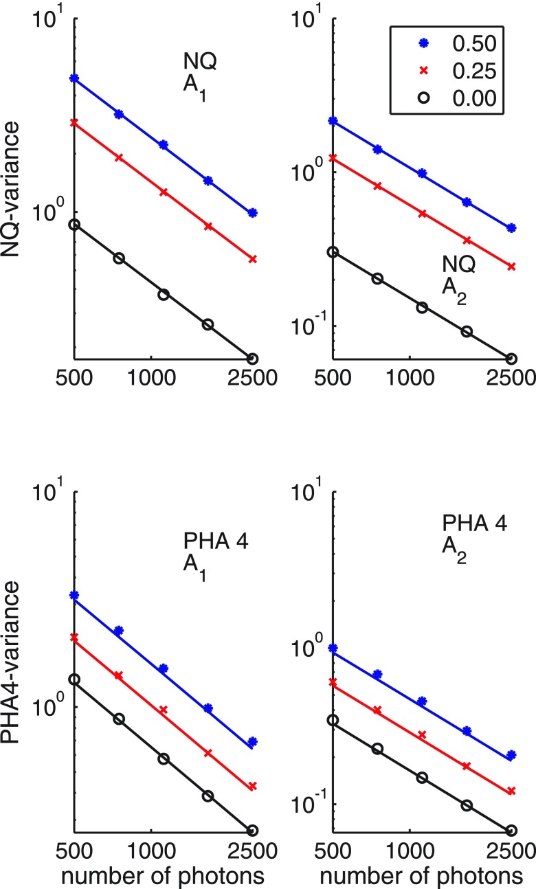
Figure 2 shows the Monte Carlo A-vector sample covariance compared to the CRLB for NQ and PHA detectors as described in Sec. 2.K. The results were compared for three values of the dead time parameter η and five values of the number of photons incident on the detector as shown in the figure.

FIG. 2.

Monte Carlo validation of theoretical formulas for noise and spectrum with pileup in Tables I and II. The graphs compare the A-vector sample covariance to the CRLB for NQ and detectors with PHA. A-vectors were computed from random measurement data as described in Sec. 2.K for three values of the dead time parameter η, 0, 0.25, and 0.5 counts per dead time, as a function of the expected number of photons incident on the detector. The individual points are the Monte Carlo values while the solid lines are the theoretical CRLB. The top panels are the A₁ and A₂ variances of the NQ detector. The bottom panels are for four bin PHA. The scales are logarithmic.

3.B. SNR vs dead time

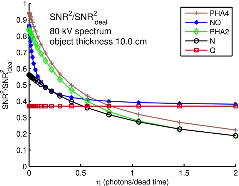
Figure 3 shows the SNR as a function of the expected number of photons incident on the detector per dead time, η. For each detector, the SNR is normalized by dividing by the ideal, complete spectrum information SNR. As discussed in Sec. 2.D, the integrated energy is assumed to be unaffected by pulse pileup so its SNR is constant.

FIG. 3.

SNR vs dead time for different detectors. The SNR is normalized by dividing by the optimal, full energy information SNR. The horizontal axis is the average number of photons incident on the detector per dead time, η. The detectors are conventional energy integrating (Q), photon counting (N), and counting with two and four bin PHA (PHA2, PHA4). An 80 kV x-ray tube spectrum is incident on the 10 cm thick, soft tissue object.

Table III lists the values of η so the SNR of the detectors is equal to the SNR of the energy integrating detector.

TABLE III.

Values of η so SNR = SNR_Q.

N	0.52
PHA2	0.65
PHA4	0.78

3.C. Increase in A-vector variance with dead time

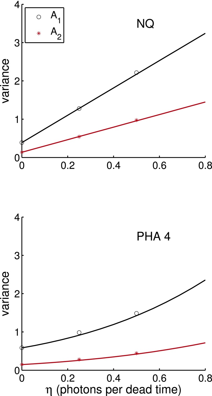
The data from the Monte Carlo simulation described in Sec. 2.K can be used to compute the increase in the A-vector noise variance as dead time increases. The results are shown in Fig. 4.

FIG. 4.

The increase in the A-vector noise variance with dead time for NQ and four bin PHA detectors. The solid lines are the theoretical CRLB variance and the individual symbols are the Monte Carlo simulation values. The NQ variances are always larger than the PHA4 variances and the ratio increases with dead time.

3.D. Effect of optimal PHA bins on SNR

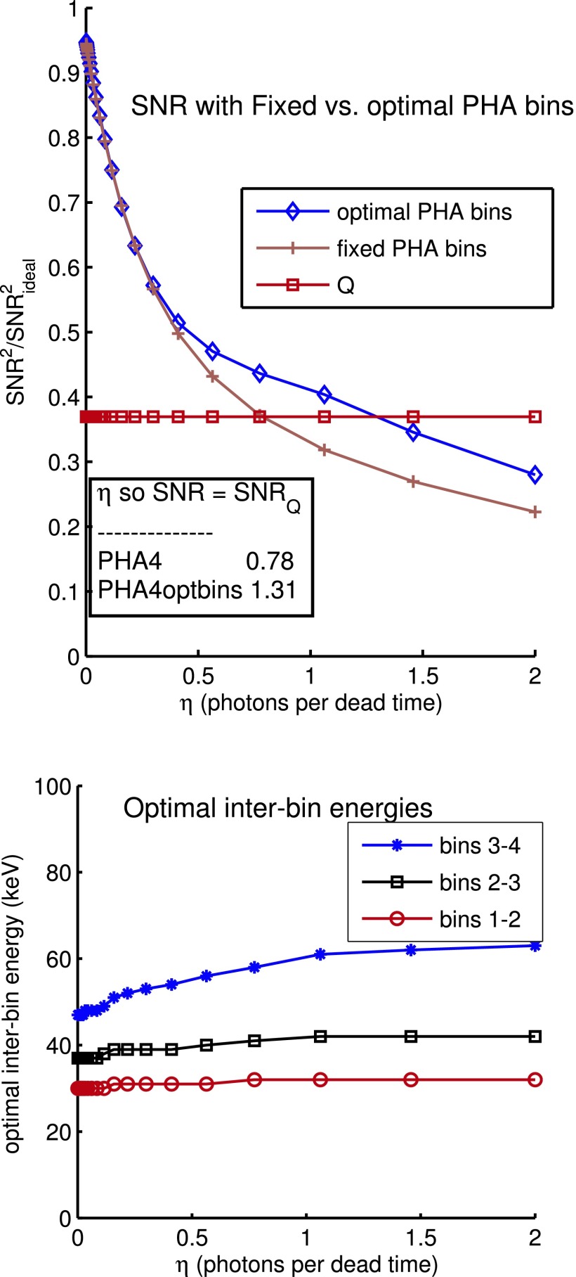
Figure 5 shows the effect of optimizing PHA bins on the SNR of a detector with four bin PHA. Plotted in the top panel is the SNR with bins optimized for each dead time individually and with fixed bins optimized for zero dead time. Also plotted for comparison is the SNR of a conventional, energy integrating detector. The inset table shows the values of η so the SNR of the PHA detector is equal to energy integrating SNR. The bottom panel shows the optimal interbin energies as a function of η.

FIG. 5.

SNR with optimal vs fixed bins. Shown in the top panel is the normalized SNR as a function of η for a counting detector with four bin PHA with optimal energy bins for every η compared with fixed bins optimized for η = 0. Also shown for reference is the SNR of a conventional energy integrating detector and a table of the values where the SNR of the PHA detector is equal to the conventional detector SNR. The bottom panel shows the optimal interbin energies.

4. DISCUSSION

The results in Fig. 3 show that the SNR decreases rapidly as the expected number of incident photons per dead time,η, increases. The decrease in SNR depends on the type of detector. The NQ detector drops more rapidly than the counting and PHA detectors while the energy integrating detector SNR is constant. Interestingly, the NQ SNR is always greater than or equal to the photon counting or energy integrating detectors since it utilizes both of these signals simultaneously.

For large enough η, the SNR of the PHA and photon counting systems becomes smaller than that of a conventional energy integrating detector. Table III shows that the values of η where the SNR drops below that of the conventional detector range from approximately 0.5 to 0.8 photons per dead time. Above these values, the energy selective data have become sufficiently degraded that they do not provide a SNR advantage over the conventional detector. These thresholds understate the effects of pileup since most of the decrease in SNR occurs at smaller values of η.

The decrease in SNR implies a stringent limit on the dead time for the count rates found in medical x-ray systems. For example, a count rate of more than 10⁸ counts/s can occur with a 1 mm² detector in low attenuation regions of abdominal CT scans.⁷ With this rate, the maximum dead time for η less than one is 10 ns. The body transmission in abdominal scans can be 10⁻² or smaller so the allowable dead time in the center of the abdomen is inverse proportionally longer. It may be possible to develop algorithms that compensate for the pileup errors in the unobstructed and low attenuation parts of the body while utilizing the more accurate data from higher attenuation regions directly.

Another way to measure the effect of pulse pileup is its effect on the A-vector noise variance. Figure 4 shows that, with the NQ detector, the noise variance increases by factors of approximately 3 and 5 for the A₁ and A₂ components as η increases from 0 to 0.8 photons per dead time. With four bin PHA data, the increase is approximately 2 and 4 times. The NQ variance increases more rapidly than that of the PHA detector.

Figure 5 shows the increase in the SNR with optimal PHA bins for each value of the dead time parameter. Although adjusting the bins for each η is physically unrealistic since the object attenuation and therefore the incident photon count rate is unknown before the measurement, the difference in the fixed vs optimal PHA bins SNR gives insight on the effect of the bin selection. The results show that there is an improvement with the value of η for SNR equal to the energy integrating SNR increasing from 0.78 to 1.31. However, the increased SNR occurs principally at larger values of η where it has already been substantially degraded. The figure also shows that the optimal interbin energies increase as η increases. This is reasonable as the recorded energies increase with pileup since they may include the energies of more than one photon.

With the idealized model, we can derive analytic formulas for the noise and spectrum with pileup, which are summarized in Tables I and II. The validity of the formulas was tested with the Monte Carlo simulation described in Sec. 2.K. For the test, the covariance of A-vector data computed from random NQ and PHA measurement data was compared to the CRLB derived from the theoretical formulas. Figure 2 shows that the Monte Carlo covariance and the CRLB agree well for the tested values of η and incident photon counts.

The model used in this paper focuses on the fundamental effects of pileup and quantum noise. Other defects occurring in photon counting detectors^2,4 such as incomplete photon energy measurement due to K radiation escape and Compton scattering, charge sharing and trapping, polarization, and other effects degrade the signals even further so the results presented tend to be an upper limit on the performance of energy selective systems. Postprocessing algorithms² may be able to compensate for detector defects but advances will most probably be limited by improvements in detector technology that reduce the defects and dead time.

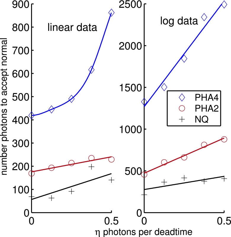
Appendix A shows that the multivariate normal distribution is acceptable for counts above approximately 3000 for logarithm data. The number of counts required increases as the number of PHA bins increases indicating that the number of counts per bin affects the distribution. Experimental tests of the probability distribution of integrated energy signals from commercial CT scanners are described by Wang et al.²⁹ and Whiting et al.³⁰ They show that normal model is accurate for large photon numbers. Wang et al.²⁹ showed that, as expected, the data failed the Shapiro–Wilk normality test for highly attenuating regions with low photon counts. However, in those cases, they found that the normal distribution still described the experimental data better than alternatives including the Poisson.

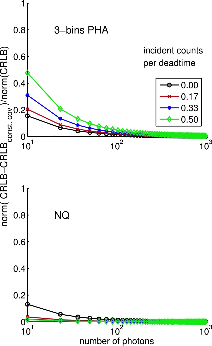
As shown in Appendix B, the CRLB with pileup is well approximated by the constant covariance formula in Eq. (7) for counts greater than 100. Since counts greater than this number are required in material-selective medical applications, the use of the constant covariance formula is justified to analyze these systems. The constant covariance formula is relatively simple to compute and is also useful to derive closed form analytical results.

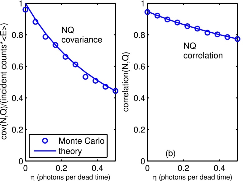
The formula for the covariance of NQ detector data with pileup derived in Appendix C agrees well with Monte Carlo simulated data. The results show that the positive correlation of the two quantities decreases rapidly as dead time increases. This correlation is important for energy selective processing and the decrease leads to the rapid decrease in SNR with pileup.

5. CONCLUSION

An idealized model of photon counting detectors is introduced that focuses on the fundamental effects of pileup and quantum noise in energy selective x-ray imaging systems. The model is used to compare the effects of pileup on SNR with different types of detectors. The SNR values were compared with the ideal full spectrum SNR and also with the SNR of conventional photon counting and energy integrating detectors. In all detectors, the SNR decreases rapidly as dead time increases. It becomes less than the SNR of a conventional energy integrating detector for values of the number of incident photons per dead time less than 1. This decrease places stringent limits on allowable dead times with the high count rates required for medical imaging systems. The probability distribution of the idealized data with pileup is shown to be accurately described as a multivariate normal for expected counts greater than those typically utilized in material-selective medical imaging systems. The constant covariance approximation to the CRLB is also shown to be valid in this case. A new formula for the covariance of the NQ detector with pileup is derived and validated.

APPENDIX A: PROBABILITY DISTRIBUTION OF PHOTON COUNT DATA WITH PILEUP

The probability distribution of the logarithm x-ray photon count and integrated energy data without pileup is usually modeled as a multivariate normal if the mean counts are sufficiently large. The statistics with pulse pileup are sufficiently different from standard counting statistics that a quantitative test of this assumption with pileup data is useful. Monte Carlo data generated, as described in Sec. 2.K, were tested with Royston’s³¹ multivariate extension of the Shapiro–Wilk test.³² The Royston multivariate algorithm is applicable for samples up to approximately 2000. The matlab function roystest,³³ which is based on Royston’s algorithm, was used with random samples of photon count and energy integral data with pileup.

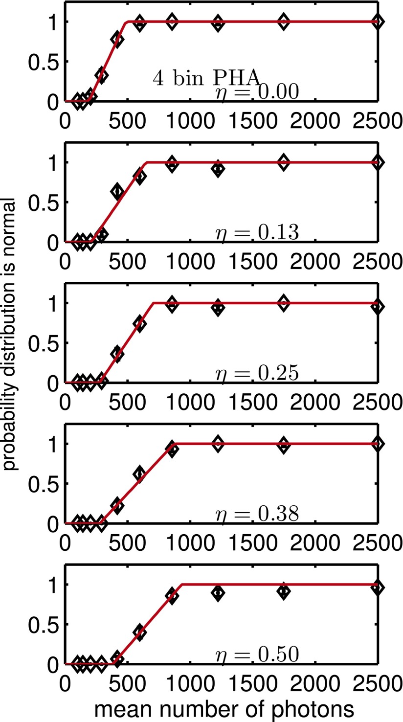
The Royston algorithm is a hypothesis test and the results are themselves random variables since they depend on the random data. In order to smooth the random results, they were averaged over a set of 50 Monte Carlo trials with 1000 samples of measurement data and plotted as a function of the mean number of photons for several values of the dead time parameter η. Figure 6 shows typical results where a 1 is assigned to the positive result that the distribution is normal and a 0 to the negative result.

FIG. 6.

Results of tests for multivariate normal for four bin PHA data for several values of the expected incident counts per dead time parameter, η, as a function of the number of photons per measurement. The y-axis is the probability that the distribution is normal. The points are the average of five trials and the error bars are the expected error. The solid line is the best fit sigmoid curve.

In general, we would expect that the data have a non-normal distribution for smaller mean counts and a more normal distribution for larger counts. Therefore, the hypothesis test averages would be near zero for small counts and near one for large counts. To estimate the minimum number of photons required for a normal distribution, a sigmoid function was fit to the average hypothesis test data and the minimum counts was the number where the sigmoid passes through 0.5. Figure 7 shows the minimum counts to accept the normal hypothesis as a function of the dead time parameter, η, for several detector types.

FIG. 7.

Minimum counts to accept the normal hypothesis. The left panel is for linear data and the right panel is for logarithm data. The detector types are two and four bin pulse height analysis, PHA2 and PHA4, and simultaneous photon counts and integrated energy, NQ. The data show random fluctuations about the fitted smooth curves.

APPENDIX B: THE CONSTANT COVARIANCE APPROXIMATION TO THE CRLB WITH PULSE PILEUP

Kay¹⁷ shows that the CRLB with a multivariate normal distribution is the inverse of the Fisher information matrix whose i, j element is

$${\displaystyle {\left[\mathbf{I}\left(\mathbf{A}\right)\right]}_{ij}={\left[\frac{\partial \mathbf{L}\left(\mathbf{A}\right)}{\partial A_i}\right]}^T{\mathbf{C}}_{\mathbf{L}}^{-1}\left[\frac{\partial \mathbf{L}\left(\mathbf{A}\right)}{\partial A_j}\right]+\frac{1}{2}tr\left[{\mathbf{C}}_{\mathbf{L}}^{-1}\frac{\partial {\mathbf{C}}_{\mathbf{L}}}{\partial A_i}{\mathbf{C}}_{\mathbf{L}}^{-1}\frac{\partial {\mathbf{C}}_{\mathbf{L}}}{\partial A_j}\right].}$$ (B1)

A previous paper¹⁵ showed that with no pileup the first term in Eq. (B1) becomes much larger than the second as the photon count increases. This term corresponds to a constant covariance and leads to Eq. (7) as the CRLB.

Evaluating the derivative terms in Eq. (B1) for the case with pileup as described in Sec. 2.J, we can compute the fractional error

$${\displaystyle \mathrm{frac}.\mathrm{err}.=\frac{‖{\mathbf{C}}_{\mathbf{A},\mathbf{CRLB}}-{\mathbf{C}}_{\mathbf{A},\mathbf{CRLB},\mathbf{const}\mathbf{cov}}‖}{‖{\mathbf{C}}_{\mathbf{A},\mathbf{CRLB}}‖}}$$ (B2)

using the constant covariance approximation to the CRLB with pileup. The symbol ‖‖ denotes a matrix norm. The results in Fig. 8 show that the error is also negligible for the photon counts typically used with material-selective medical x-ray imaging systems.

FIG. 8.

CRLB error using constant covariance formula ${\mathbf{C}}_{\mathbf{A},\mathbf{CRLB}}=\left({\mathbf{M}}^{\mathbf{T}}{\mathbf{C}}_{\mathbf{L}}^{-1}\mathbf{M}\right)$. The fractional error given by Eq. (B2) is plotted as a function of the mean number of counts for four values of the dead time parameter η. The top panel shows the error with three bin PHA while the bottom panel is for the NQ detector.

APPENDIX C: THE NQ COVARIANCE WITH PILEUP

For any two random variables, the covariance is

$${\displaystyle \mathrm{cov}\left(N_{\mathrm{rec}},Q\right)=〈N_{\mathrm{rec}}Q〉-〈N_{\mathrm{rec}}〉〈Q〉.}$$ (C1)

The expected value of the product in Eq. (C1) can be evaluated with conditional expectation

$${\displaystyle 〈N_{\mathrm{rec}}Q〉={〈N_{\mathrm{rec}}〈Q{|}_{N_{\mathrm{rec}}=n_{\mathrm{rec}}}〉〉}_{n_{\mathrm{rec}}}.}$$ (C2)

Since Q is the sum of the energy of the incident photons

$${\displaystyle 〈Q{|}_{N_{\mathrm{rec}}=n}〉=\sum _{k=1}^{〈N|n_{\mathrm{nrec}}〉}{E}_k,}$$ (C3)

where $〈N|n_{\mathrm{rec}}〉$ is the expected value of the number of incident photons given that n_rec are recorded. Inverting Eq. (10) for λ = ρt = N,

$${\displaystyle 〈N|n_{\mathrm{rec}}〉=\left(1+\eta \right)n_{\mathrm{rec}}.}$$ (C4)

Since the E_k are independent and identically distributed, the expected value of Eq. (C3) is

$${\displaystyle 〈〈Q{|}_{N_{\mathrm{rec}}=n_{\mathrm{rec}}}〉〉=〈N|n_{\mathrm{rec}}〉〈E〉=\left(1+\eta \right)n_{\mathrm{rec}}〈E〉.}$$

Using this in Eq. (C2),

$${\displaystyle 〈N_{\mathrm{rec}}Q〉=\left(1+\eta \right)〈N_{\mathrm{rec}}^2〉〈E〉.}$$ (C5)

We can use the general formula $\text{Var}\left(\mathbf{X}\right)=〈{\mathbf{X}}^2〉-{〈\mathbf{X}〉}^2$ and Eqs. (10) and (11) to show that

$${\displaystyle 〈N_{\mathrm{rec}}^2〉=\mathrm{var}\left(N_{\mathrm{rec}}\right)+{〈N_{\mathrm{rec}}〉}^2=\frac{\lambda }{{\left(1+\eta \right)}^3}+\frac{{\lambda }^2}{{\left(1+\eta \right)}^2}.}$$ (C6)

Substituting in Eq. (C5) and using the result in Eq. (C1)

$${\displaystyle \mathrm{cov}\left(N_{\mathrm{rec}},Q\right)=\frac{\lambda 〈E〉}{{\left(1+\eta \right)}^2}.}$$ (C7)

Equation (C7) was validated with 10 000 random NQ data values generated as described in Sec. 2.K. The results in Fig. 9 show that the theoretical formula accurately describes the covariance of the simulated data.

FIG. 9.

Covariance and correlation of NQ detector data with pulse pileup. The Monte Carlo data are the individual points and the theoretical formulas are the solid lines. Note that the data are positively correlated but the correlation decreases as η increases.

REFERENCES

- 1.Aslund M., Fredenberg E., Telman M., and Danielsson M., “Detectors for the future of x-ray imaging,” Radiat. Prot. Dosim. 139, 327–333 (2010). 10.1093/rpd/ncq074 [DOI] [PubMed] [Google Scholar]
- 2.Taguchi K. and Iwanczyk J. S., “Vision 20/20: Single photon counting x-ray detectors in medical imaging,” Med. Phys. 40, 100901 (19pp.) (2013). 10.1118/1.4820371 [DOI] [PMC free article] [PubMed] [Google Scholar]
- 3.Knoll G. F., Radiation Detection and Measurement, 3rd ed. (Wiley, Hoboken, NJ, 2000), Ch. 17. [Google Scholar]
- 4.Overdick M., Baumer C., Engel K. J., Fink J., Herrmann C., Kruger H., Simon M., Steadman R., and Zeitler G., “Towards direct conversion detectors for medical imaging with x-rays,” IEEE Trans. Nucl. Sci. NSS08, 1527–1535 (2008). 10.1109/NSSMIC.2008.4775117 [DOI] [Google Scholar]
- 5.Schlomka J. P., Roessl E., Dorscheid R., Dill S., Martens G., Istel T., Bäumer C., Herrmann C., Steadman R., Zeitler G., Livne A., and Proksa R., “Experimental feasibility of multi-energy photon-counting K-edge imaging in pre-clinical computed tomography,” Phys. Med. Biol. 53, 4031–4047 (2008). 10.1088/0031-9155/53/15/002 [DOI] [PubMed] [Google Scholar]
- 6.Shikhaliev P. M., “Energy-resolved computed tomography: First experimental results,” Phys. Med. Biol. 53, 5595–5613 (2008). 10.1088/0031-9155/53/20/002 [DOI] [PubMed] [Google Scholar]
- 7.Iwanczyk J. S., Nygard E., Meirav O., Arenson J., Barber W. C., Hartsough N. E., Malakhov N., and Wessel J. C., “Photon counting energy dispersive detector arrays for x-ray imaging,” IEEE Trans. Nucl. Sci. 56(3), 535–542 (2009). 10.1109/TNS.2009.2013709 [DOI] [PMC free article] [PubMed] [Google Scholar]
- 8.Taguchi K., Zhang M., Frey E. C., Wang X., Iwanczyk J. S., Nygard E., Hartsough N. E., Tsui B. M. W., and Barber W. C., “Modeling the performance of a photon counting x-ray detector for CT: Energy response and pulse pileup effects,” Med. Phys. 38, 1089–1102 (2011). 10.1118/1.3539602 [DOI] [PMC free article] [PubMed] [Google Scholar]
- 9.Wang A. S., Harrison D., Lobastov V., and Tkaczyk J. E., “Pulse pileup statistics for energy discriminating photon counting x-ray detectors,” Med. Phys. 38, 4265–4275 (2011). 10.1118/1.3592932 [DOI] [PubMed] [Google Scholar]
- 10.Barrett H. H. and Myers K., Foundations of Image Science (Wiley-Interscience, Hoboken, NJ, 2003), Chap. 11. [Google Scholar]
- 11.Alvarez R. E., “Near optimal energy selective x-ray imaging system performance with simple detectors,” Med. Phys. 37, 822–841 (2010). 10.1118/1.3284538 [DOI] [PMC free article] [PubMed] [Google Scholar]
- 12.Tapiovaara M. J. and Wagner R., “SNR and DQE analysis of broad spectrum x-ray imaging,” Phys. Med. Biol. 30, 519–529 (1985). 10.1088/0031-9155/30/6/002 [DOI] [Google Scholar]
- 13.Overdick M., Ruetten W., and Zaengel T., “X-ray detector having a large dynamic range,” U.S. patent 6,759,658 (July 6, 2004).
- 14.Roessl E., Ziegler A., and Proksa R., “On the influence of noise correlations in measurement data on basis image noise in dual-energy like x-ray imaging,” Med. Phys. 34, 959–966 (2007). 10.1118/1.2514058 [DOI] [PubMed] [Google Scholar]
- 15.Alvarez R. E., “Dimensionality and noise in energy selective x-ray imaging,” Med. Phys. 40, 111909 (13pp.) (2013). 10.1118/1.4824057 [DOI] [PMC free article] [PubMed] [Google Scholar]
- 16.Alvarez R. E. and Macovski A., “Energy-selective reconstructions in x-ray computerized tomography,” Phys. Med. Biol. 21, 733–744 (1976). 10.1088/0031-9155/21/5/002 [DOI] [PubMed] [Google Scholar]
- 17.Kay S. M., Fundamentals of Statistical Signal Processing: Estimation Theory (Prentice Hall PTR, Upper Saddle River, NJ, 1993), Vol. 1 , Chap. 4. [Google Scholar]
- 18.Wielopolski L. and Gardner R. P., “Prediction of the pulse-height spectral distortion caused by the peak pile-up effect,” Nucl. Instrum. Methods 133(2), 303–309 (1976). 10.1016/0029-554X(76)90623-6 [DOI] [Google Scholar]
- 19.Yu D. F. and Fessler J. A., “Mean and variance of single photon counting with deadtime,” Phys. Med. Biol. 45, 2043–2056 (2000). 10.1088/0031-9155/45/7/324 [DOI] [PubMed] [Google Scholar]
- 20.Ross S. M., A First Course in Probability, 5th ed. (Prentice Hall College Div, New York, NY, 1997), Sec. 6.3. [Google Scholar]
- 21.Ross S. M., A First Course in Probability, 5th ed. (Prentice Hall College Div, New York, NY, 1997), Sec. 5.5. [Google Scholar]
- 22.Ross S. M., Stochastic Processes, 2nd ed. (Wiley, New York, NY, 1995), Sec. 3.3. [Google Scholar]
- 23.Frey E. C., Wang X., Du Y., Taguchi K., Xu J., and Tsui B. M. W., “Investigation of the use of photon counting x-ray detectors with energy discrimination capability for material decomposition in micro-computed tomography,” Proc. SPIE 6510, 65100A (2007). 10.1117/12.711711 [DOI] [Google Scholar]
- 24.Ross S. M., Simulation, Fourth Edition, 4th ed. (Academic, New York, NY: ), Sec. 5.1. [Google Scholar]
- 25.Boone J. M. and Seibert J. A., “An accurate method for computer-generating tungsten anode x-ray spectra from 30 to 140 kV,” Med. Phys. 24, 1661–1670 (1997). 10.1118/1.597953 [DOI] [PubMed] [Google Scholar]
- 26.Hubbell J. H. and Seltzer S. M., “Tables of x-ray mass attenuation coefficients and mass energy-absorption coefficients,” National Institute of Standards and Technology (online) (2014) (available URL: http://physics.nist.gov/PhysRefData/XrayMassCoef/cover.html).
- 27.“ICRU, Report 44: Tissue substitutes in radiation dosimetry and measurement,” International Commission on Radiological Units and Measurements (online) (2014) (available URL: http://www.icru.org).
- 28.van den Bos A., Parameter Estimation for Scientists and Engineers (Wiley-Interscience, Hoboken, NJ, 2007), Sec. 5.3. [Google Scholar]
- 29.Wang J., Lu H., Liang Z., Eremina D., Zhang G., Wang S., Chen J., and Manzione J., “An experimental study on the noise properties of x-ray CT sinogram data in Radon space,” Phys. Med. Biol. 53, 3327–3341 (2008). 10.1088/0031-9155/53/12/018 [DOI] [PMC free article] [PubMed] [Google Scholar]
- 30.Whiting B. R., Massoumzadeh P., Earl O. A., O’Sullivan J. A., Snyder D. L., and Williamson J. F., “Properties of preprocessed sinogram data in x-ray computed tomography,” Med. Phys. 33, 3290–3303 (2006). 10.1118/1.2230762 [DOI] [PubMed] [Google Scholar]
- 31.Royston J. P., “Some Techniques for Assessing Multivarate Normality Based on the Shapiro- Wilk W,” J. R. Stat. Soc. Ser. C Appl. Stat. 32(2), 121–133 (1983). [Google Scholar]
- 32.Shapiro S. S. and Wilk M. B., “An analysis of variance test for normality (complete samples),” Biometrika 52(3–4), 591–611 (1965). 10.1093/biomet/52.3-4.591 [DOI] [Google Scholar]
- 33.Trujillo-Ortiz A., Hernandez-Walls R., Barba-Rojo K., and Cupul-Magana L., “Roystest: Royston’s multivariate normality test. A matlab file” (online) (2014) (available URL: matlab Central File Exchange, http://www.mathworks.com/matlabcentral/fileexchange/17811).