An Application of Serially Balanced Designs for the Study of Known Taste Samples with the α-ASTREE Electronic Tongue

Abstract

The α-ASTREE e-Tongue instrument uses seven sensors to characterize taste signals associated with a liquid sample. The instrument was used to study eight test preparations (comprised of a blank, four preparations corresponding to four known tastes and Sodium Topiramate in three concentrations known to have a bitter taste) and eight washes. Serially balanced residual effects designs were used to order the samples to estimate residual and main effects. The design provided for eight repeated measurements per test preparation. The experimental results suggested the following: (1) The seven sensors can be separated into three groups according to the ability to discriminate test preparations, and three of the sensors contributed little or no information. Further investigation suggested the lack of differentiability might be due to the age of the sensors. (2) The sensors discriminated known tastes from blank. The residual effect due to test preparations might appear after repeated usage. (3) Exploratory principal component analysis of the data indicated that nearly 90% of the total variability across the seven sensors could be explained by a single principal component. (4) The four standard taste preparations did not correspond to orthogonal dimensions in the principal component axes. (5) The three Sodium Topiramate test preparations could neither be associated with the corresponding known bitter taste sample nor could the three doses be shown to follow a quantitative dose-response relationship on the e-Tongue measurement scale. The practical interpretation of the results of the statistical analysis indicates only poor discriminative ability of the e-Tongue to distinguish clearly between increasing concentrations of a known bitter compound such as Sodium Topiramate. No apparent linear relationship could be discerned over increasing concentrations that would allow the quantification of bitterness.

INTRODUCTION

There are about 10,000 taste buds residing on the surface of the tongue which are involved in taste perception (1). Different parts of the tongue are sensitive to different flavors with bitterness sensitive taste buds located toward the back of the tongue. Besides bitterness, sweetness, sourness, saltiness, and umami are the other basic tastes. The perception of taste is also affected by temperature and texture, as well as psychological factors (bad childhood memory, acculturation). Subjective evaluation of taste through human sensory tests is well known (2,3); however, the quantification and characterization of tastes by means of objective instruments is a recent development.

In pharmaceutical development, the taste of oral formulations is an important consideration. Children and elderly patients in particular are highly sensitive to a drug’s bitter taste which may make more difficult or even prevent a patient from completing a therapeutic course of treatment. Therefore, the early identification of the bitterness potential of a drug formulation is an important goal in drug development. An important practical concern is the design of human studies for taste testing of pharmaceutical compounds. Pharmaceutical compounds during early development must obtain a license through the investigational new drug (IND) process if intended for human clinical trials necessary to gain approval for marketing. Consequently, during the development phase when formulation development is exploring the taste properties of the new compound, any taste testing experiment must be carried out as a regular clinical study adhering to Food and Drug Administration (FDA) requirements governing the use of an IND. This means the writing of a clinical protocol, tracking of medical status and side effects, and filling out a detailed case report form followed by a comprehensive clinical report. A medical monitor has to supervise the dosing. The administrative burden in carrying out a taste study in humans of a pharmaceutical compound is much more than in a taste panel evaluation of a food product. Therefore, an objective electronic device which could replace humans for the study of bitterness would be of great practical benefit to the pharmaceutical industry. In this paper, we discuss our results researching the use of one such instrument for this purpose.

THE α-ASTREE e-TONGUE

The α-ASTREE e-Tongue instrument was developed in 2000 and marketed by the French Company Alpha M.O.S. (4). It has found wide application in the food and beverage industry and only recently have pharmaceutical applications emerged. The instrument contains seven sensors, each of which produces an electrical signal related to the chemical composition of the test solution. The combination of the responses from the seven sensors constitutes the essential measurement for the objective assessment of taste (5). Zhu et al. (6) reported that the e-Tongue could successfully distinguish different tastes, and Uchida et al. (7) reported that the instrument could discern bitterness associated with different chemicals. Principal component analysis (PCA), discriminant factorial analysis (DFA), and partial least squares (PLS) were among the statistical methods used to describe the relationship between the sensors and test preparations (1,8–10); however, none of these papers considered the possibility of order or carryover effects from consecutive immersions of the sensors, which could conceivably lead to biased signals even with the use of intervening washes. A statistical design that would mitigate this possibility is an important feature of the experiments we carried out.

The e-Tongue instrument can be seen as a robotic device in which the samples are presented in a serial order. This ordering raises the possibility that the residual of one sample may be carried to subsequent samples. One cannot discount this possibility even with intervening washes since the wash vessels can become increasingly more contaminated by repeated washings. Although these effects may be small, the statistical analysis must consider the possibility of these carryover effects to avoid biasing the results.

PCA and DFA have been used to cluster different taste samples; however, the question of quantifying the intensity of the taste (bitterness in particular) on the scale of the axes produced by the principal components requires a case by case study. Linear regression and PLS have been used to model and predict different bitterness intensity scores (i.e., from low to high) for single chemicals, but different chemicals corresponding to the same taste may not share a common location or direction on the axes or have similar dose-response relationships. Consequently, the notion of similarity in dose-response curves as a paradigm for objectively assessing taste through an instrument as understood in the bioassay framework was an important question for us.

Therefore, as a first step to addressing the stated goal, it was necessary to characterize the output of the sensors in relation to known standard test preparations using serially balanced statistical designs (11,12). These designs permit the estimation of carryover effects as well as direct effects due to test preparations. The inherent structure of the data was investigated using linear regression and subsequent principal component analysis and cluster analysis. The results of our experiments are presented as summaries of what relationships we found between the output of the sensors and the test preparations.

METHOD

Data Description and Design of Experiment

The experiment involved two groups of samples, where the first group was composed of the following test preparations:

• C0 = distilled water,

• C1 = Sodium Topiramate 0.5 mg/ml in water (low bitterness drug concentration),

• C2 = Sodium Topiramate 5 mg/ml in water (middle bitterness drug concentration),

• C3 = Sodium Topiramate 10 mg/ml in water (high bitterness drug concentration),

• S1 = 0.01 mM HCl in water (standard sourness taste),

• S2 = 0.01 mM NaCl in water (standard saltiness taste),

• S3 = 0.01 mM monosodium glutamate in water (standard umami taste),

• S4 = 1 mM quinine hydrochloride in water (standard bitterness taste),

The second group was composed of eight washes designated W1, W2, …, W8. Each test preparation from group 1 was followed by a wash from group 2. The question of how the preparations should be sequentially ordered arose, since residual or carryover contamination from repeated immersions of the seven sensors could be present. In this case, the sequence requires preparations from one group to follow samples from another group (i.e., a wash step has to be performed between test preparations from group 1), and consequently, the ordering must be performed in such a way as to accommodate this requirement. The ordering followed the construction of serially balanced sequences as given in Altan et al. (11,12). Essentially, the method of construction depends on appropriately linking the entries of a Williams design (13) into a chain and interweaving the entries from a Latin square design between the consecutive entries of the chain defined by the Williams design. To illustrate how it works, we start with a Williams design of order eight for the eight samples of group 1, as shown in Fig. 1. For the sake of simplicity, we replace the sample names of C1-S4 by 0–7. Omitting the 0th row, we form four chains of equal size by interweaving the entries as indicated by the dotted lines. Here B1–B4 are the beginnings of the chains and E1–E4 are the ends. Augment 0 to the very beginning to obtain a type 2 sequence:

• 0 17263545362710 37465647302120 57675041323140 70615243425160.

Fig. 1.

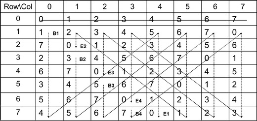
Illustration of the construction of a serially balanced sequence with eight treatments

Then, repeat each sample once to obtain the type 1 sequence:

• 0 1726354553627110 3746564733002120 5767750413223140 7066152434425160.

The eight washes of group 2 are inserted into the above type 1 sequence according to the row-column designation of an 8 × 8 Latin square design.

Final design consisted of a sequence of samples and washes of length 128 + 1 (corresponding to positions 0, 1, 2, …, 128). Each test preparation and wash was evaluated eight times with C0 evaluated nine times to permit residual effect balancing. The different sensors are designated AB, BB, ZZ, JE, DA, BA, and CA and their immersions into the test samples followed the serial order discussed previously. The observed responses formed a 129 × 7 data matrix.

Statistical Analysis

Modeling Analysis

The following linear model with terms corresponding to the experimental design factors was fitted to the observations from each sensor:

$${\mathit{\gamma }}_{\mathit{i}}=\mathit{\mu }+{\mathit{I}}_{\mathit{i}}\times \left\{{\mathit{\tau }}_{{\mathit{d}}_{\mathit{i}}}+{\mathit{\Delta }}_{{\mathit{g}}_{\mathit{i}-2}}^{*}+{\mathit{\Delta }}_{{\mathit{d}}_{\mathit{i}-2}}^{*}\right\}+\left(1-{\mathit{I}}_{\mathit{i}}\right)\left\{{\mathit{\rho }}_{{\mathit{g}}_{\mathit{i}}}+{\mathit{\gamma }}_{{\mathit{d}}_{\mathit{i}-1}}+{\mathit{\gamma }}_{{\mathit{g}}_{\mathit{i}-2}}^{*}\right\}+{\mathit{\epsilon }}_{\mathit{i}}$$ 1

• Where y_i = response at ith position,

• μ = overall mean,

• I_i = $\left\{\begin{array}{cc}\hfill 1\hfill & \hfill \mathrm{if}\mathit{i}\mathrm{th}\mathrm{position}\mathrm{is}\mathrm{a}\mathrm{test}\mathrm{sample}\hfill \\ \hfill 0\hfill & \hfill \mathrm{if}\mathit{i}\mathrm{th}\mathrm{position}\mathrm{is}\mathrm{a}\mathrm{wash}\hfill \end{array}\right.,$

• ${\mathit{\tau }}_{{\mathit{d}}_{\mathit{i}}}$ = direct effect of test sample d_i at ith position,

• ${\mathit{\Delta }}_{{\mathit{g}}_{\mathit{i}-1}}$ = residual effect of wash g_i−1 from (i−1)th position (first order),

• ${\mathit{\Delta }}_{{\mathit{d}}_{\mathit{i}-2}}^{*}$ = residual effect of test sample d_i−2 from (i−2)th position (second order),

• ${\mathit{\rho }}_{{\mathit{g}}_{\mathit{i}}}$ = direct effect of wash g_i at ith position,

• ${\mathit{\gamma }}_{{\mathit{d}}_{\mathit{i}-1}}$ = residual effect of test sample d_i−1 from (i−1)th position (first order),

• ${\mathit{\gamma }}_{{\mathit{g}}_{1-2}}^{*}$ = residual effect of wash g_i−2 from (i−2)th position (second order).

ε_i is residual error assumed normally and independently distributed. Model (1) was used to estimate the direct effects of test preparations and washes, the first-order residual effects of washes on test preparations and test preparations on washes, and the second-order residual effects of test preparations on test preparations and washes on washes. Because there was no residual effect on the first sample of the sequence, it was removed from the model fitting. Least squares means (LSMs) for each test preparation and wash were estimated by sensor, forming a 16 × 7 matrix to be used for principal component analysis and cluster analysis. The reason to use LSMs for subsequent analyses but not the original observations was that it represents the essential sufficient statistics accounting for the effects of the model (1) parameters, thus capturing in a concise way the information contained across the 128 repeated measurements of the sequence.

Principal Component Analysis

Principal component analysis is a statistical method whose purpose is to reduce the dimensionality of multivariate data. In this case, we have seven sensors providing responses to four known standard taste samples: sourness (HCL), saltiness (NaCL), umami (Na glutamate), and bitterness (quinine). A second and equally important goal was to relate known concentrations of a bitter tasting drug (Sodium Topiramate) to the measured responses of these standard taste samples. The measurements by the seven sensors form a multivariate response. The translation of the global responses of the sensors to each basic taste sample would ideally fall on distinct principal components related to the human perception of taste expressed through the responses of the four standard taste samples. The wash samples would fall in the proximity of the origin on the principal component axes, and their dispersion around the origin would represent the space of no effect.

The calculations were carried out on the covariance matrix of the LSMs using S-PLUS® (Version 8.0) princomp() function.

Cluster Analysis

Cluster analysis is a collection of statistical methods that identifies groups of individuals or objects that are more similar to each other than to individuals from other groups. The algorithms of cluster analysis are broadly classified into hierarchical and non-hierarchical algorithms. In this article, the hierarchical procedures were carried out, in which a hierarchy or tree-like structure was constructed to illustrate the relationship among individuals. Specifically, the single linkage method (nearest neighbor) was used to calculate the distance between clusters. The clustering tree is grown according to the minimum distance between clusters which can be interpreted as the degree of similarity between subjects/clusters: the deeper the leaf, the greater the similarity. In the ideal situation, the group of test preparations would fall in a cluster that is completely separated from the group of washes. Within the cluster of test preparations, different tastes would be grouped according to their similarity in sensor readings.

The analysis was carried out on the LSMs using the SAS® (Version 9.1) PROC CLUSTER procedure.

RESULT AND DISCUSSION

Data Visualization

Figure 2 shows the responses of test preparations from each sensor. According to the ability to differentiate test preparations, the sensors might be roughly categorized into three groups:

1. Sensors ZZ and CA had the greatest differentiability. There was a clear separation between test preparations with the magnitude generally following the same order. The correlation coefficient between ZZ and CA was 0.95.

2. Reponses of test preparations from sensors AB and BA fell in a very narrow range with no separation at all. The correlation coefficient between AB and BA was 0.89.

3. The remaining three sensors, BB, JE, and DA might have some ability for detecting different test preparations, but not as strong as ZZ and CA.

Fig. 2.

Scatter plot of the observed responses of test samples by sensor

The three-group pattern observed for the test preparations was somewhat surprisingly reflected but to a lesser degree in the responses of washes, as shown in Fig. 3.

Fig. 3.

Scatter plot of the observed responses of wash samples by sensor

Significance of Effects

The LSMs calculated from model (1) are given in Table I by test preparation and sensor along with results of significance testing of test preparations (compared to C0) and of washes (compared to each other). Pairwise significance testing was conducted at level p = 0.05 with a Bonferroni adjustment for multiplicity, p = 0.05/7 = 0.007. The following conclusions were drawn:

1. No direct or residual effects were attributed to washes.

2. No direct or residual effects were found for sensor AB, BA, and DA, except for a second-order residual effect of test sample S1 (0.01 mM HCL) for sensor BA. This could be artifactual.

3. For sensors CA, ZZ, JE, and BB, direct effects against C0 (water) for test preparations were frequently found significant. First-order residual effects of test preparations on washes were found significant occasionally, and a second-order residual effect of test preparation S1 was found significant for sensor BB. This finding may be artifactual, but it may also indicate instrument biases.

Table I.

Least Squares Means (LSMs) by Test Sample and Sensor (units of 10²)

	Sensor
Sample	CA	ZZ	AB	BA	DA	JE	BB
C0	14.4	13.8	7.4	8.5	12.8	9.7	9.7
C1	19.3*	23.0*	7.4	8.5	11.1	9.5	6.0*
C2	19.3*	22.9*	7.4	8.3	11.5	9.4	6.1*
C3	22.3*	26.0*+	7.2	7.8	8.7	8.2*	3.5*
S1	−0.6*+	2.6*	7.2	7.8#	9.3	4.4*+	1.0*+#
S2	6.5*	9.6*	7.3	8.1	10.8	6.1*+	5.0*
S3	14.9	18.5*	7.4	8.4	9.5	8.7	4.7*
S4	8.8*	12.1	7.4	8.5	12.8	6.6*	7.2
W1	15.9	18.9	7.6	8.9	13.3	10.1	8.6
W2	14.5	17.7	7.2	7.9	10.9	9.0	8.0
W3	15.6	18.2	7.7	9.1	13.7	10.0	9.6
W4	13.7	16.5	7.0	7.4	10.8	8.7	7.2
W5	15.8	18.0	7.3	7.9	10.6	9.8	7.3
W6	14.5	15.8	7.3	8.3	12.9	9.3	8.6
W7	16.6	17.1	7.2	8.0	13.7	9.6	8.6
W8	14.5	15.8	7.5	8.5	13.2	9.3	8.9
Range of Std Error	0.6	0.6–0.7	0.14–0.15	0.3–0.4	0.9–1.0	0.2	0.5–0.6

^*Significantly different direct treatment effect compared to C0 of a test sample, or different from one or more washes of a wash

⁺Significantly different first-order residual effect compared to C0 of a test sample, or different from one or more washes of a wash

^#Significantly different second-order residual effect compared to C0 of a test sample, or different from one or more washes of a wash

Some discriminative ability to distinguish test preparations from washes was found although sensors AB, BA, and DA specifically could not distinguish known test preparations from control (C0). It is clear that these three sensors were non-informative in relation to estimating direct effects in our experiment. Removing these three sensors from the calculation of the LSMs generated from model (1) would not affect the essential features of the principal component analysis and cluster analysis.

Principal Components

The principal component analysis was performed on the 7 × 7 covariance matrix of the LSMs. The results indicated that the first component explained nearly 87% of the total variance and the second about 12%. Figure 4 shows an enhanced plot of the location of the test preparations and washes on the first two principal components axes. We found that

1. The washes formed a distinct group as expected. The control (C0) was very close to the washes since they were basically the same. All other test preparations were displaced from the washes which were related to direct treatment effects of the test preparations.

2. The four standard taste samples were clearly distinguishable on the two-dimensional scale as far as relative location, but it was seen that S4 (standard bitterness taste) was in the quadrant opposite to C1, C2, and C3 (known bitter drug), which implied the sensors could distinguish between the four tastes, but bitterness as a sensory quality arising from different chemical compounds could fall in very different locations on the two-dimensional PC axes. It is possible that another bitter tasting compound may fall in yet another location in relation to the PC axes found in our experiment.

3. The sensors could not distinguish between C1 (low concentration) and C2 (middle concentration), but C1 and C2 were clearly separated from C3 (high concentration). One possible explanation is that the intensity signal of bitterness that the sensors could pick up depends on a threshold factor with no broad monotonic relationship to concentration.

4. Compared to what is seen in Fig. 4, the relative location of each test preparation did not change much with the removal of sensors AB, BA, and DA, as given in Fig. 5. This again confirmed these three sensors only added noise to the experiment.

Fig. 4.

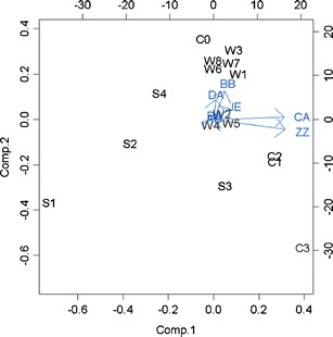
Biplot of the first principal component vs. the second principal component displaying the importance of the sensors and the relative locations of the test samples and washes

Fig. 5.

Biplot of the first principal component vs. the second principal component displaying the importance of the sensors and the relative locations of the test samples and washes, with the removal of sensors AB, BA, and DA

Our interpretation of the relative locations of the test preparations and washes on the two-dimensional plot is that human sensory testing would still be required to both characterize and quantify the perception of bitterness. The data does not support the ability of the instrument to serve as an unconditional replacement for human sensory judgment. Similarity assumption in the bioassay sense between the known standard bitter compound quinine and the bitter drug samples did not hold in our experiment.

Clusters

The cluster analysis was carried out on the LSMs. One of the primary goals in a cluster analysis is to determine the number of groups. Typically, one looks for natural groupings defined by long stems. Figure 6 shows the clustering tree generated from the cluster analysis. If we cut the tree at the minimum distance of 0.4, then clearly, the washes and the control C0 form one major cluster, with test preparation S3 (umami taste) joining as the last candidate. The level of similarity within this major cluster is pretty consistent. The rest of the test preparations forms individual clusters with C1 and C2 joining together in high similarity. The findings were consistent with the results from the principal component analysis. In addition, the cluster analysis provided quantitative similarity measurement. The structure of the tree remained the same after removing the three non-informative sensors AB, BA, and DA, as shown in Fig. 7.

Fig. 6.

Clustering tree displaying the order of grouping for test and wash samples

Fig. 7.

Clustering tree displaying the order of grouping for test and wash samples, with the removal of sensors AB, BA, and DA

CONCLUSIONS

The results of our experiments studying the α-ASTREE Electronic Tongue for test preparation differentiation using a serially balanced statistical design found several sensors were non-informative. We could not find numerical criteria corresponding to separate principal components between test preparations corresponding to known tastes or varying levels of bitterness. Graphical visualization of the e-Tongue signals by sensor and test preparation did not indicate a clear criterion permitting discrimination between known taste samples in relation to the independent dimensions in the PCA. It is recommended that a multi-laboratory Gage R&R study be carried out to characterize the repeatability and reproducibility of the instrument in assessing and characterizing a set of standardized test preparations corresponding to varying concentrations of known bitter compounds from different chemical classes. Correlations to a standard taste panel would also be desirable. The results of such a study should be made available to researchers interested in pursuing experiments utilizing the instrument.

REFERENCES

- 1.Murray OJ, Dang W, Bergstrom D. Using an electronic tongue to optimize taste-masking in a lyophilized orally disintegrating tablet formulation. Pharm Tech. 2004;28:42–52. [Google Scholar]
- 2.Gacula MC, Jr, Singh J, Bi J, Altan S. Statistical methods in good and consumer research. 2. Burlington: Academic; 2009. pp. 25–74. [Google Scholar]
- 3.Malisa M, Breimer M, Sadik OA. Electronic-noses and sensory array-based systems: design and application. Proceedings of the 5th international symposium on olfaction and the electronic-nose. Lancaster: Technomic Publ. Co; 1999. pp. 27–42. [Google Scholar]
- 4.Electronic nose and tongue, Alpha M.O.S. Newsl. 2004.
- 5.Miyanaga Y, Inoue N, Ohnishi A, Fujisawa E, Yamaguchi M, Uchida T. Quantitative prediction of the bitterness suppression of elemental diets by various flavors using a taste sensor. Pharm Res. 2003;20(12):1932–8. doi: 10.1023/B:PHAM.0000008039.59875.4f. [DOI] [PubMed] [Google Scholar]
- 6.Zhu L, Seburg RA, Tsai E, Puech S, Mifsud J. Flavor analysis in a pharmaceutical oral solution formulation using an electronic-nose. J Pharm Biomed Anal. 2003;34(3):453–61. doi: 10.1016/S0731-7085(03)00651-4. [DOI] [PubMed] [Google Scholar]
- 7.Uchida T, Tanigake A, Miyanaga Y, Matsuyama K, Kunitomo M, Kobayashi Y, et al. Evaluation of the bitterness of antibiotics using a taste sensor. J Pharm Pharmacol. 2003;55(11):1479–85. doi: 10.1211/0022357022106. [DOI] [PubMed] [Google Scholar]
- 8.Isz, S., Poling, J., The e-tongue in the pharmaceutical industry: a fast and objective method for taste masking and the selection of best tasting formulations. AAPS Show Daily. 2003.
- 9.Vlasov Y, Legin A, Rudnitskaya A. Electronic tongues and their analytical application. Anal Bioanal Chem. 2002;373(3):136–46. doi: 10.1007/s00216-002-1310-2. [DOI] [PubMed] [Google Scholar]
- 10.Zhu, L., Seburg. R.A., Thompson, K., Tsai, E., Isz, S., Feasibility study of an electronic-tongue for potential pharmaceutical applications. Present Am Chem Soc (ACS) Annu Meet. 2004.
- 11.Altan S, Manola A, Pandey R, Troisis J, Ragahavarao D. A statistical design consideration in robotic systems. Drug Inf J. 2004;38(3):283–7. [Google Scholar]
- 12.Altan S, Ragahavarao D. Serially balanced designs for two sets of treatments. J Biopharm Stat. 2005;15(2):279–82. doi: 10.1081/BIP-200049829. [DOI] [PubMed] [Google Scholar]
- 13.Jones B, Kenward MG. Design and analysis of cross-over trials. London: Chapman and Hall; 1989. [Google Scholar]