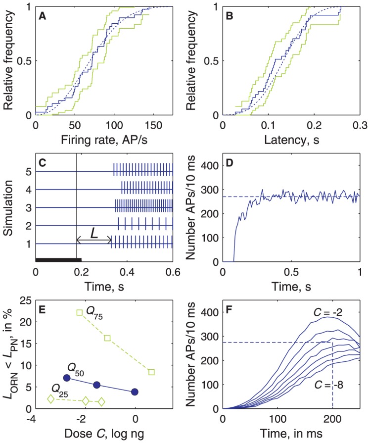
Figure 9. Model of a large ORN population converging on a small PN population.

(A, B) Example at dose C = 1 log ng of cumulated distributions of modelled firing rates (A) and latencies (B) of ORNs and comparison with experimental data. Distributions of experimental values (N = 32, same as in Fig. 5A, B) shown as staircase graphs (solid line) with 95% confidence intervals (green lines). Distributions of modelled F and L shown as smooth curves (in blue) based on N = 5 000 drawings. Firing rates in the model obey eq. 4 and latencies eq. 8 with parameters L ₀, ln(λ), L _m, F _M, C _1/2, ln(n) drawn from a multinormal distribution with their observed means, SDs and correlations (S5 Table). The modelled and experimental distributions are not significantly different (Kolmogorov–Smirnov tests at level 1%). (C) Examples of 5 simulated ORN responses with interspike interval 1/F and latency L at C = 1 log ng for 5 parameter drawings; 7000 such responses are summated to simulate the whole ORN population). (D) Simulated spontaneous activity of the whole ORN population (based on the lognormal distribution with μ = 1.23 and σ = 0.71 shown in Fig. 3E); the firing rate fluctuates around a stationary value ∼270 AP/10 ms. (E) Proportion of ORNs that respond with a shorter latency than the typical PN (with all 6 parameters equal to their median values; solid line), than a slow and insensitive PN (parameters equal to their 75% quantiles, dotted), and than a fast and sensitive PN (parameters equal to their 25% quantiles; dashed) at doses C ₀, C _1/2 and C _s. (F) PSTH of the total number of spikes fired per 10 ms at doses from −8 to −2 log ng by a simulated population of 7000 NROs. The summated firing rate close to detection threshold (dotted line, 275 APs per 10 ms, see text) is reached for C≈−4.5 log ng at time ∼200 ms.