Evaluating Variables as Unbiased Proxies for Other Measures

Abstract

To assess validity of a low-intensity measure of fitness (X) in a population of older adults as a proxy measure for the original, high-intensity measure (Y), we used ordinary least square regression with the new, potential proxy measure (X) as the sole explanatory variable for Y. A perfect proxy measure would be unbiased (i.e., result in a regression line with a y-intercept of zero and a slope of one) with no error (variance equal to zero). We evaluated the properties of potential biases of proxy measures. A two degree-of-freedom approach using a contrast matrix in the setting of simple linear ordinary least squares regression was compared to a one degree-of-freedom paired t test alternative approach. We found that substantial improvements in power could be gained through use of the two degree-of-freedom approach in many settings, while scenarios where no linear bias was present there could be modest gains from the paired t test approach. In general, the advantages of the two degree-of-freedom approach outweighed the benefits of the one degree-of-freedom approach. Using the two degree-of-freedom approach, we assessed the data from our motivating example and found that the low-intensity fitness measure was biased, and thus was not a good proxy for the original, high-intensity measure of fitness in older adults.

1. Introduction

Proxy measures evaluation has been presented in the context where a true, underlying measure may be unobservable, so this measure may be replaced by an observable proxy (e.g., Kotz & Johnson, 1986, p. 323; Trenkler & Stahlecker, 1996; Hawkins, 2002). It is often of interest of scientific investigators to develop a new measure to serve as a proxy for another in the setting where the original is observable. Proxy measures can be of great importance, particularly when costs, broadly defined, are substantially less for measuring the new proxy compared to the original measure. A systematic review by Dickinson, Hrisos, Eccles, Francis and Johnston (2010), however, found problems with methods frequently used to evaluate proxy measures.

The focus of this work was on the evaluation of whether a new measure, X, served as a good proxy for the original measure Y. We evaluated the proxy for the setting where Y∣X was (at least approximately) a continuous measure. In the Methods section that follows, we first defined our criteria for assessing whether a measure serves as a valid proxy. We used simple linear regression of Y onto X to provide a formal means to assess for validity as a proxy, and compared this approach to a simpler strategy of taking the difference between measures for each subject, and testing the null hypothesis that the mean of these differences is zero using a paired t test.

The motivating example was the assessment of a lower-impact, self-paced, submaximal step test (the Step Test Exercise Prescription, or STEP test; Petrella, Koval, Cunningham & Paterson, 1998; Petrella Koval, Cunningham & Paterson, 2001; Petrella & Wight, 2000) as a proxy for the rigorous, maximal, high-intensity peak oxygen consumption (VO₂ peak) test to measure fitness levels. More specifically, we were interested in the validity of this potential proxy in an older population than had been previously examined that included subjects with Alzheimer’s Disease (Vidoni et al., 2013). A major research focus of The University of Kansas Alzheimer’s Disease Center (KU ADC), which is funded by the National Institute on Aging, is on modifiable lifestyle risk factors and Alzheimer’s Disease prevention. Thus, a submaximal fitness assessment could serve as a key measure of interest for research at the KU ADC. Discussions compared and contrasted these two approaches for assessing proxy measures in general settings, and conclusions from our motivating example were presented.

2. Methods

For a variable, X, to serve as a valid proxy measure for another (the original) variable, Y, the relationship between these two variables would be approximately Y = X. In a simple linear regression framework, this relationship would ideally be (Y∣X = x) = x + E, where E represents the random error and most of the distribution of E falls at or near zero (Kotz & Johnson, 1986, p. 323). A normal distribution for E with a mean of zero and small variance parameter meets these criteria; and is also advantageous given the wealth of literature on the theory and practice of ordinary least squares regression that fit under this simple linear regression paradigm (e.g., Draper & Smith, 1998, chap. 1; Kleinbaum, Kupper, Muller & Nizam, 1998, chap. 5; Kutner, Nachtsheim & Neter, 2004, chap. 1), though as noted by Lin (1989), settings where the variance of E is large may be problematic for this approach. Bell-shaped distributed errors seem plausible for the difference between two measures—regardless of the underlying distributions of the individual random variables X and Y—if Y indeed is a valid proxy for X. It is noteworthy that the assumptions of this model did not require both Y and X to be continuous, so long as the conditional distribution of Y∣X is approximately normally distributed.

We formally defined the model using the simple linear regression paradigm for assessment of X as a proxy measure for Y as

$$(Y\mid X=x)={\beta }_0+{\beta }_{1}x+E$$ (1)

where E~N(0, σ²). As noted above, one of our properties of a valid proxy was a small variance; however, the property of unbiasedness in and of itself may be important, for example in some clinical settings, where there is motivation to report a proxy without adjustment. Hence, the focus of this work was on the property of the unbiasedness of the proxy measure; specifically, that β₀ = 0 ∩ β₁ = 1 in (1). To formally test the null hypothesis that H₀: β₀ = 0 ∩ β₁ = 1, we used a contrast matrix to perform the simultaneous, two degree-of-freedom test.

2.1 Linear Transformation

To facilitate the two approaches investigated, we first re-parameterized this two degree-of-freedom approach using a linear transformation. From (1), we subtracted the observed value of X (i.e., x) to define the random variable, Z₁∣X, or

$$\begin{array}{c}(Z_1\mid X=x)=(Y-X\mid X=x)={\beta }_0+{\beta }_{1}x-x+E\\ (Z_1\mid X=x)={\beta }_0+({\beta }_1-1)x+E.\end{array}$$ (2a)

Re-labeling the parameters yielded

$$(Z_1\mid X=x)={\gamma }_0+{\gamma }_{1}x+E.$$ (2b)

From (2b), assessment for unbiasedness of the proxy measure as β₀ = 0 ∩ β₁ = 1 in (1) was equivalent to testing. γ₀ = γ₁ = 0. Under the assumptions defined above regarding the error, E~N(0, σ²), testing for unbiasedness can be done by comparing

$$F=\frac{{(\widehat{\underset{¯}{\gamma }}-\underset{¯}{\gamma })}^T(\widehat{\underset{¯}{\gamma }}-\underset{¯}{\gamma })/2}{{(\underset{¯}{z_1}-X\widehat{\underset{¯}{\gamma }})}^T(\underset{¯}{z_1}-X\widehat{\underset{¯}{\gamma }})/(n-2)},$$ (3a)

where γ̱, which represented the true, unknown parameters (γ₀, γ₁)^T, to a central F-distribution with two and n– 2 degrees of freedom in the numerator and denominator, respectively (e.g., using Rencher, 2000, pp. 184-190). In (3a), $\underset{¯}{z_1}$ represented the observed vector of differences between the n original (Y) and proxy (X) measures, and γ̱̂ the ordinary least squares maximum likelihood estimates (MLEs) for γ̱. In the Appendix we demonstrated that this analogous transformed approach produced equivalent inferences as γ̂₀ = β̂₀ and γ̂₁ = β̂₁ − 1.

To test for unbiasedness we defined the null hypothesis as H₀:γ̱ = 0̱, which yielded

$$F=\frac{{\widehat{\underset{¯}{\gamma }}}^T\widehat{\underset{¯}{\gamma }}/2}{{(\underset{¯}{z_1}-X\widehat{\underset{¯}{\gamma }})}^T(\underset{¯}{z_1}-X\widehat{\underset{¯}{\gamma }})/(n-2)}.$$ (3b)

Under the alternative hypothesis, γ̱ ≠ 0̱ (i.e., the proxy was not valid as the proxy was a biased measure of the original), the distribution of F (3b) followed a non-central F-distribution with non-centrality parameter

$$\lambda ={\underset{¯}{\gamma }}^T{X}^T{X}_{\underset{¯}{\gamma }}/2{\sigma }^2=(n{\gamma }_0^2+2n\overline{x}{\gamma }_0{\gamma }_1+{\gamma }_1^2{\underset{¯}{x}}^T\underset{¯}{x})/2{\sigma }^2$$ (4a)

(Rencher, 2000, p. 185). This followed from the fact that the contrast matrix was the identity matrix for testing this null hypothesis. We further refined (4a) by substituting for x̱^Tx̱ using the formula for the sample variance of the proxy measure (X),

$${\underset{¯}{x}}^T\underset{¯}{x}=(n-1)S^2+n{\overline{x}}^2,$$

which yielded

$$\lambda =\{n{\gamma }_0^2+2n\overline{x}{\gamma }_0{\gamma }_1+{\gamma }_1^2[(n-1)S_x^2+n{\overline{x}}^2]\}/2{\sigma }^2.$$ (4b)

[The subscript was added to $S_x^2$ in (4b) to more clearly indicate it as the sample variance from the proxy measure, X, which represented the explanatory variable in underlying models of (1) and (2b).]

2.2 Paired t Test Approach

We evaluated an alternative approach for assessing whether the proxy measure was biased (and therefore not a valid proxy) by conducting the one-sample paired t-test on (Z₂∣X = x), which from (2a) was defined as (Y − X∣X = x). In contrast to the model used by (2a), this alternative approach excluded the linear term (γ₁) altogether. The test for unbiasedness to assess the validity of the proxy measure was similarly constructed as in (3a-b). However, the design matrix on the right hand side of the equation, X* (say), was equal to the n × 1 vector 1̱; thus, the MLE γ̱̂* (say) for this alternative approach was the scalar ${\left({\underset{¯}{1}}^T\underset{¯}{1}\right)}^{-1}{\underset{¯}{1}}^T\underset{¯}{z_2}={\overline{z}}_2$. The true, unknown mean parameter vector was also a scalar, so

$${\underset{¯}{\gamma }}^{\ast }={\gamma }^{\ast }={\gamma }_0+{\gamma }_1\overline{x}$$

where γ₀ and γ₁ were the same parameters from the model of (2b) (Rencher, 2000, p 154). This resulted in

$$F^{\ast }=\frac{{({\widehat{\underset{¯}{\gamma }}}^{\ast }-{\underset{¯}{\gamma }}^{\ast })}^T({\widehat{\underset{¯}{\gamma }}}^{\ast }-{\underset{¯}{\gamma }}^{\ast })/1}{{(\underset{¯}{z_2}-X{\widehat{\underset{¯}{\gamma }}}^{\ast })}^T(\underset{¯}{z_2}-X{\widehat{\underset{¯}{\gamma }}}^{\ast })/(n-1)}=\frac{(n-1){({\overline{z}}_2-{\gamma }_0-{\gamma }_1\overline{x})}^2}{{(\underset{¯}{z_2}-{\overline{z}}_2\underset{¯}{1})}^T(\underset{¯}{z_2}-{\overline{z}}_2\underset{¯}{1})},$$ (5a)

which was compared to a central F-distribution with one and n − 1 degrees of freedom in the numerator and denominator, respectively. To test for unbiasedness under this paired one-sample t test approach we defined the null hypothesis as

$$H_0:{\gamma }^{\ast }=0\iff {\gamma }_0+{\gamma }_1\overline{x}=0\iff {\gamma }_0=-{\gamma }_1\overline{x},$$

which yielded

$$F^{\ast }=\frac{(n-1){\overline{z}}_2^2}{{\left(\underset{¯}{z_2}-{\overline{z}}_2\underset{¯}{1}\right)}^T\left(\underset{¯}{z_2}-{\overline{z}}_2\underset{¯}{1}\right)}.$$ (5b)

Under the alternative hypothesis, γ* ≠ 0 (i.e., the proxy was not valid as it was a biased measure of the original), the distribution of F* (5b) followed a non-central F-distribution with non-centrality parameter

$${\lambda }^{\ast }=n{({\gamma }_0+{\gamma }_1\overline{x})}^2/2{\sigma }^2$$ (6)

(Rencher, 2000, p. 185). This followed from the fact that the contrast matrix was the scalar value of one for this null hypothesis. Of note, the null hypothesis for this paired t test approach, H₀: γ₀ = −γ₁x̄, indicated it would be unable, in some settings, to reject the null hypothesis of a biased proxy even when it was truly biased (i.e., γ₀ ≠ 0 ∪ γ₁ ≠ 0). This represented a potential shortcoming of the paired t test approach.

2.3 Power of the Two Approaches

From (3b), (4b), (5b), and (6), power functions were derived based on a given design matrix. Specifically, the probability of rejecting the null hypothesis (that X was a valid proxy for Y because it was unbiased) when in fact it was not unbiased followed a non-central F_2.n−2.λ distribution, and for the alternative approach it followed a non-central F_1.n−1.λ* distribution. The non-centrality parameters (λ and λ*) were functions of the true parameters γ₀, γ₁, [or analogously β₀ and β₁ using the form of (1)], σ², n, and x̄. For the initial proposed approach (with two degrees of freedom in the numerator), λ was also a function of $S_x^2$ Expanding the polynomial term in λ* and using substitution, we wrote λ as

$$\lambda ={\lambda }^{\ast }+\left(n-1\right)S_x^2{\gamma }_1^2/2{\sigma }^2.$$

Writing the non-centrality parameter, λ, in this way implied power advantages in the proposed two degree-of-freedom approach to detect linear deviations from unbiasedness, particularly: 1) when there was more variation in the proxy measure collected (X) as quantified by $S_x^2$; or 2) when the absolute value of γ₁ was large (assuming a sample size of n > 1). However, when these values were small relative to σ² (the variance in the differences given X), the non-centrality parameter λ approached that of λ*, which gave potential advantage to the paired t test approach based on the differences in the degrees of freedom for the respective F tests.

To facilitate our comparison of the theoretical results for these two approaches, a receiver operating characteristics (ROC) curve approach was used similar to that done in Mahnken, Wick, Gajewski and Mayo (2010). Specifically, we plotted the type I error along the horizontal axis and the power on the vertical axis. Notably, in the setting of the valid proxy actually being unbiased (i.e., when the null H₀: γ₀ = γ₁ = 0 was true) the power was expected to equal to the type I error, and so both approaches were anticipated to produce identical curves in this setting where the power equaled the type I error.

3. Motivating Example

A cohort of 102 adult research participants was recruited through the KU ADC Registry cohort and a concurrent study in the Research in Exercise and Cardiovascular Health (REACH) Laboratory (Billinger, van Swearingen, McClain, Lentz & Good, 2012). The protocols for obtaining the original (Y, VO₂ peak) and proxy (X, STEP) measures were described in Vidoni et al. (2013). While differences in the KU ADC Registry and REACH Laboratory measure collections differed slightly as described by Vidoni et al., these data provide a useful example for the statistical discussions presented here. Further, we treated all subjects from the two study sources as homogeneous for our motivating example sections below. Approval was provided for both parent studies that obtained the source data measures by The University of Kansas Medical Center Human Subjects Committee (#11132 and #12460).

Simple linear regression was used to assess the STEP test (X) as an unbiased proxy for VO₂ peak (Y). The GLM procedure in SAS version 9.3 (SAS Institute Inc., Cary, NC, 2002-2010) was used for this analysis. To test for unbiasedness of our proxy measure, we used the form γ₀ = γ₁ = 0 for our null hypothesis corresponding to (2b). This enabled the use of the CONTRAST statement within the GLM procedure, which limited hypothesis testing to be subject to the constraint

$$L{\underset{¯}{\beta }}_0=\underset{¯}{0}.$$

For our hypothesis, this was only the case using the linear transformation approach [i.e., the model of (2b)]. As stated above and demonstrated in the Appendix, this linear transformation approach produced identical inferences for corresponding hypothesis tests. Model assessment by residual analysis was not further described nor their results presented as this was not the focus of the work presented here. More formal presentation of the motivating example results, including subgroup-specific assessments, was presented previously in Vidoni et al. (2013). The alternative, paired t test approach was also performed for comparison.

4. Results

Plots were generated to compare the power curves using an ROC curve approach. This enabled comparisons of power across varying levels of type I error. While presented over the entire range of [0, 1], the focus of the results will often be around those portions of the plots with lower type I error. Curves were generated with varying values of β₀ and β₁ of -0.25(0.25)0.25 and 0.75(0.25)1.25, respectively such that they spanned null and alternative hypotheses—including non-null cases where the paired t test approach fit for testing the true, underlying model. The effect of the variance, σ², of the original model (1) was held fixed at one across all models.

4.1 Power as a Function of x̄

Sample mean (X̄) values for the proxy measures (X) varied within each plot in Figure 1 from -1(1)1. In each case where the slope parameter was not equal to one (i.e., where the alternative approach under-fit the relationship between the original and its proxy) the proposed (two degree-of-freedom) approach outperformed or did no worse than the alternative paired t test (one degree-of-freedom) approach. This was demonstrated by the dashed curves being closer to the point coordinate (0, 1) on the plots than the correspondingly-colored solid curves, or the two corresponding curves overlaying one another. In the cases where there was no linear bias in the proxy measure (i.e., where β₁ = 1), the one degree-of-freedom paired t test approach outperformed the two degree-of-freedom approach except in the case where the proxy was completely unbiased. In this latter case (i.e., where β₀ = 0 and β₁ = 1) the non-centrality parameters λ and λ* where both equal to zero, so the power had a 1:1 relationship with the type I error in that case.

Figure 1.

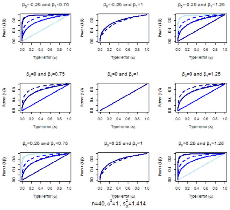
Comparison of the two degree-of-freedom (dashed) versus one degree-of-freedom, paired t test (solid) approach over x̄ = −1, 0, and 1 (light to dark)

Note. Underlying model y_i = β₀ + β₁ x_i + ε_i where ε_i ~ N(0, σ²); power and type I error correspond to the test of the null hypothesis that the proxy is not biased, which for the two degree-of-freedom approach is H₀ : β₀ = 0 ∩ β₁ = 1 and is H₀ : β₀ = −(β₁ − 1)x̄ for the one degree-of-freedom, paired t test approach

4.2 Power as a Function of $S_x^2$

Sample variance ( $S_x^2$) values for the proxy measures (X) varied within each plot in Figure 2, using values of 0.1, 1, and 2. In these plots, the power curves for the paired t test (one degree-of-freedom) approach completely overlaid one another. This followed from the fact that the non-centrality parameters for these models, λ*, were not functions of $S_x^2$ [see (6)]. We again saw a slight power advantage with the paired t test (one degree-of-freedom) approach over that of the proposed method for the cases where no linear bias was present, and both power functions reverting to the type I error rate when the new measure was an unbiased proxy for the original. A slight advantage of the paired t test approach was seen in other scenarios when the sample variance of the proxy measure was close to zero; but this advantage was lost as the sample variance increased. For the case where the bias of the proxy was only in the linear term the proposed (two degree-of-freedom) approach always outperformed the paired t test (one degree-of-freedom) approach, with the greater advantage observed as the sample variance of the proxy (X) increased.

Figure 2.

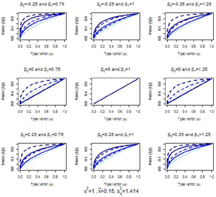
Comparison of the two degree-of-freedom (dashed) versus one degree-of-freedom, paired t test (solid) approach over n = 10, 20, and 50 (light to dark)

Note. Underlying model y_i = β₀ + β₁ x_i + ε_i where ε_i ~ N(0, σ²); power and type I error correspond to the test of the null hypothesis that the proxy is not biased, which for the two degree-of-freedom approach is H₀ : β₀ = 0 ∩ β₁ = 1 and is H₀ : β₀ = −(β₁ − 1)x̄ for the one degree-of-freedom, paired t test approach

4.3 Power as a Function of n

For the comparison of these approaches over increasing sample sizes (n; Figure 3), the proposed approached had greater power in each scenario where a linear bias was present, compared to slight advantages with the pair t test (one degree-of-freedom) approach under the settings where there was no linear bias (i.e., β₁ = 1). Also, for the paired t test approach the power did not improve as a function of sample size when the bias was only in the linear term (i.e., when β₀ = 0, but β₁ ≠ 1). As with the evaluations of power as functions of other parameters, when the proxy (X) truly was an unbiased measure of the original (Y), the type I error was preserved under either approach.

Figure 3.

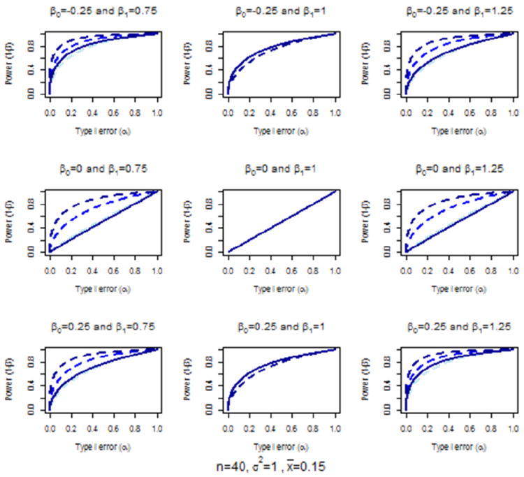
Comparison of the two degree-of-freedom (dashed) versus one degree-of-freedom, paired t tested (solid) approach over $S_x^2=0.1$, 1, and 2 and (light to dark)

Note. Underlying model where y_i = β₀ + β₁x_i + ε_i where ε_i ~ N (0, σ²) power and type I error correspond to the test of the null hypothesis that the proxy is not biased, which for the two degree-of-freedom approach is H₀ : β₀ = 0 ∩ β₁ = 1 and is H₀ : β₀ = −(β₁ − 1)x̄ for the one degree-of-freedom, paired t test approach

4.4 Assessment of the STEP Test as a Proxy for VO₂ Peak Fitness Measures

A scatter plot of the STEP test versus the VO₂ peak test was presented in Figure 4. The ordinary least squares regression line estimated from these data [of the (1) form] was plotted (solid), as was y = x a reference line (dashed). This figure indicated a general bias toward the STEP test overestimating the fitness level of the VO₂ peak testing. The maximum likelihood estimates for the original scale (1) were

$${\widehat{\beta }}_0=-5.37\mathrm{and}{\widehat{\beta }}_1=1.04;$$

or equivalently on the linear transformed scale

$${\widehat{\gamma }}_0=-5.37\mathrm{and}{\widehat{\gamma }}_1=\mathrm{0.04.}$$

Figure 4.

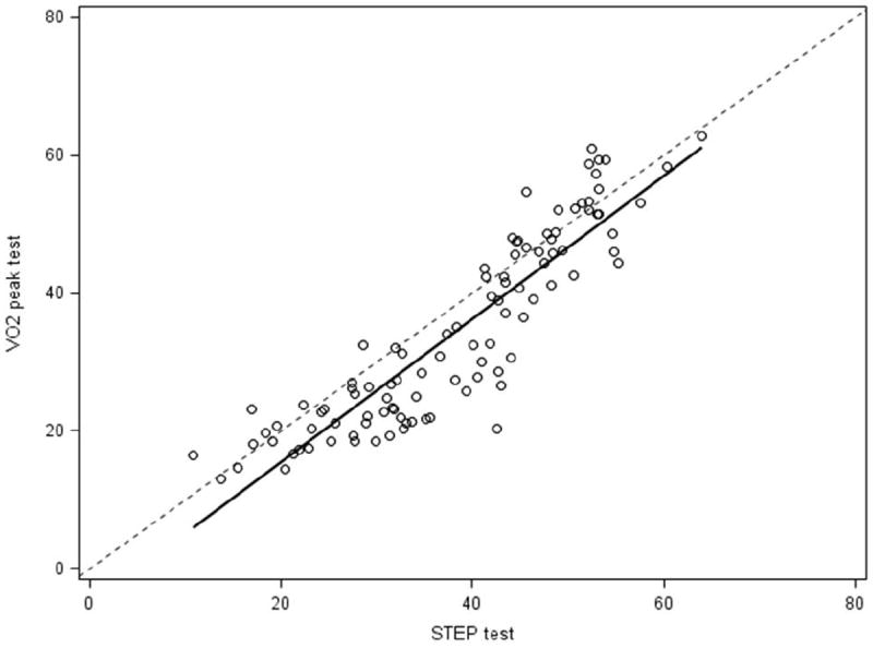
Scatter plot of the potential proxy STEP test measure by the true fitness measure VO₂ peak

The F test of the null hypothesis that the STEP measure was an unbiased proxy for VO₂ peak was rejected (p<0.0001). In this example, the alternative, paired t test approach also rejected this null hypothesis (H₀: γ* = 0; p<0.0001).

5. Discussion

Proxy measures are important tools. Less costly alternative means to assess important measures have substantial importance in scientific research, clinical practice, business, and sociology, among other areas of application. A simple approach to evaluating a measure as a proxy is to test for differences in central tendency by applying the one sample paired t test to the observed differences. However, this approach can overlook important systematic forms of bias that, when left uncheck, could lead to poorly capturing of the underlying construct of interest by use of a proxy. Previous studies of methods for evaluating proxy measures has also been described by Bland and Altman (1999) and Dickenson et al. (2010).

Our investigations demonstrated that when linear biases were present the power to detect that a measure was a poor proxy was greatly reduced with the paired t test approach. Especially notable was the fact that when the bias was entirely on the slope parameter, increases in sample size did not correspondingly increase the power of the paired t test (one degree-of-freedom) approach for detecting that the proxy was invalid due to bias (see Figure 2 plots where β₀ = 0). While the cases where there was no linear bias in the proxy indicated slight increases in power, the magnitudes were much greater for changes when the bias did, in fact, include linear effects. This advantage followed from estimating only one mean parameter for the intercept rather than two—one for the intercept and one for the slope. We were unable to find an analytic solution to the probability that the alternative, one degree-of-freedom approach would have greater power than the two degree-of-freedom approach when no linear term was needed (i.e., β₁ = 1).

As noted above, for our motivating example the conclusions did not change with the differing approaches. However, the null hypothesis of the one degree-of-freedom paired t test approach was

$$H_0:{\gamma }^{\ast }=0\iff {\gamma }_0+{\gamma }_1\overline{x}=0\iff {\gamma }_0=-{\gamma }_1\overline{x}.$$

This implied that even in the presence of strong linear bias, the null hypothesis using the one degree-of-freedom approach would not be rejected when the sample mean for the proxy (X) is nearly centered. This was highlighted by the results of Figure 1, where the one degree-of-freedom approach had power equal to the type I error for the scenarios: where x̄ = −1 for the plots where β₀ = −0.25 ∩ β₁ = 0.75 and β₀ = 0.25 ∩ β₁ = 1.25 (light blue solid lines); where x̄ = 0 for the plots where β₀ = 0 ∩ β₁ = 0.75 and β₀ = 0 ∩ β₁ = 1.25 (blue solid lines); and where x̄ = 1 for the plots where β₀ = 0.25 ∩ β₁ = 0.75 and β₀ = −0.25 ∩ β₁ = 1.25 (dark blue solid lines). In our motivating example x̄ ≈ 38, so there are an infinite number of possible (β₀, β₁) pairs that could produce values with little power to reject the null hypothesis even in cases of highly biased, poor proxy measures. These pairs would be all those that fall along the line

$${\gamma }_0=-{\gamma }_1\overline{x}\iff {\beta }_0=-({\beta }_1-1)38\iff {\beta }_0=-38{\beta }_1+38.$$

Although there are an infinite number of pairs that fall on this line, these solutions would still represent a restricted subset of the entire two-dimensional space of all possible (β₀, β₁) pairs. We further note that samples with centered proxy measures (i.e., x̄ = 0) also suffer from a power disadvantage for detecting systematic linear biases. Thus, overall, we believe these findings support the use of the two degree-of-freedom approach advocated here over the risk of a slight loss of power due to using an F_{2,n − 2} distribution as opposed to an F_{1,n − 1} distribution (paired t test approach) for inference about whether a proxy is a biased measure of the original.

Appendix

Proof of Equivalence of Inferences for γ̂₀ = β̂₀ and γ̂₁ = β̂₁ − 1

Let Y_i∣X_i = x_i ~ N(β₀ + β₁ x_i, σ²), so x_i is treated as a constant and y_i = β₀ + β₁ x_i + ε_i, where ε_i ~ N (0, σ²). The maximum likelihood estimators for β₀ and β₁ are

$${\widehat{\beta }}_0=\frac{{\sum }_i^n{y}_i}{n}-{\beta }_1\frac{{\sum }_i^n{x}_i}{n}=\overline{y}-{\beta }_1\overline{x}$$

and

$${\widehat{\beta }}_1=\frac{{\sum }_i^n{x}_i{y}_i}{{\sum }_i^n{x}_i^2}-\frac{{\beta }_o}{{\sum }_i^n{x}_i}.$$

For the transformed Z_i∣X_i, (Y_i − X_i∣X_i = x_i)~N(β₀ + [β₁ − 1] x_i, σ²), so

$$y_i-x_i={\beta }_0+[{\beta }_1-1]x_i+{\epsilon }_i,$$

where ε_i ~ N (0, σ²). Let γ₀ = β₀ and γ₁ = β₁ − 1, then

$$y_i-x_i={\gamma }_0+{\gamma }_1{x}_i+{\epsilon }_i.$$

Now to show that γ̂₀ = β̂₀,

$$\begin{array}{c}{\widehat{\gamma }}_0=\frac{{\sum }_i^n(y_i-x_i)}{n}-{\gamma }_1\frac{{\sum }_i^n{x}_i}{n}\\ {\widehat{\gamma }}_0=\frac{{\sum }_i^n{y}_i-{\sum }_i^n{x}_i}{n}-({\beta }_1-1)\frac{{\sum }_i^n{x}_i}{n}\\ {\widehat{\gamma }}_0=\overline{y}-\overline{x}-({\beta }_1\overline{x}-\overline{x})\\ {\widehat{\gamma }}_0=\overline{y}-{\beta }_1\overline{x};\end{array}$$

so γ̂₀ = β̂₀. Finally, to show that γ̂₁ = β̂₁ − 1,

$$\begin{array}{c}{\widehat{\gamma }}_1=\frac{{\sum }_i^n{x}_i(y_i-x_i)}{{\sum }_i^n{x}_i^2}-\frac{{\gamma }_o}{{\sum }_i^n{x}_i}\\ {\widehat{\gamma }}_1=\frac{{\sum }_i^n{x}_i{y}_i-{\sum }_i^n{x}_i^2}{{\sum }_i^n{x}_i^2}-\frac{{\gamma }_o}{{\sum }_i^n{x}_i}\\ {\widehat{\gamma }}_1=\frac{{\sum }_i^n{x}_i{y}_i}{{\sum }_i^n{x}_i^2}-1-\frac{{\beta }_o}{{\sum }_i^n{x}_i}\\ {\widehat{\gamma }}_1=\frac{{\sum }_i^n{x}_i{y}_i}{{\sum }_i^n{x}_i^2}-\frac{{\beta }_o}{{\sum }_i^n{x}_i}-1,\end{array}$$

so γ̂₁ = β̂₁ − 1.

References

- Billinger SA, van Swearingen E, McClain M, Lentz AA, Good MB. Recumbent stepper submaximal exercise test to predict peak oxygen uptake. Medicine and Science in Sports and Exercise. 2012;44(8):1539–1544. doi: 10.1249/MSS.0b013e31824f5be4. http://dx.doi.org/10.1249/MSS.0b013e31824f5be4. [DOI] [PMC free article] [PubMed] [Google Scholar]
- Bland JM, Altman DG. Measuring agreement in method comparison studies. Statistical Methods in Medical Research. 1999;8:135–160. doi: 10.1177/096228029900800204. http://dx.doi.org/10.1191/096228099673819272. [DOI] [PubMed] [Google Scholar]
- Dickinson HO, Hrisos S, Eccles MP, Francis J, Johnston M. Statistical considerations in a systematic review of proxy measures of clinical behavior. Implementation Science. 2010;5(20) doi: 10.1186/1748-5908-5-20. http://dx.doi.org/10.1186/1748-5908-5-20. [DOI] [PMC free article] [PubMed] [Google Scholar]
- Draper NR, Smith H. Applied regression analysis. 3. New York, NY: John Wiley & Sons, Inc; 1998. http://dx.doi.org/10.1002/9781118625590. [Google Scholar]
- Hawkins DM. Diagnostics for conformity of paired quantitative measurements. Statistics in Medicine. 2002;21:1913–1935. doi: 10.1002/sim.1013. http://dx.doi.org/10.1002/sim.1013. [DOI] [PubMed] [Google Scholar]
- Kleinbaum DG, Kupper LL, Muller KE, Nizam A. Applied regression analysis and other multivariable methods. 3. Pacific Grove, CA: Duxbury Press; 1998. [Google Scholar]
- Kotz S, Johnson NL, editors. Encyclopedia of statistical sciences. Vol. 7. New York, NY: John Wiley & Sons; 1986. [Google Scholar]
- Kutner MH, Nachtsheim CJ, Neter J. Applied linear regression models. 4. Boston, MA: McGraw-Hill Irwin; 2004. [Google Scholar]
- Lin LI-K. A concordance coefficient to evaluate reproducibility. Biometrics. 1989;45(1):255–268. http://dx.doi.org/10.2307/2532051. [PubMed] [Google Scholar]
- Mahnken JD, Wick JA, Gajewski BJ, Mayo MS. A study design with conditional, serially assessed co-primary endpoints: an application to a single-arm, pilot non-Hodgkin’s lymphoma trial. Drug Development Research. 2010;71:395–403. http://dx.doi.org/10.1002/ddr.20387. [Google Scholar]
- Petrella R, Koval J, Cunningham D, Paterson D. Predicting VO2max in community dwelling seniors using a self-paced step test. Medicine and Science in Sports and Exercise. 1998;30(5):76. http://dx.doi.org/10.1097/00005768-199805001-00433. [Google Scholar]
- Petrella RJ, Koval JJ, Cunningham DA, Paterson DH. A self-paced step test to predict aerobic fitness in older adults in the primary care clinic. Journal of the American Geriatrics Society. 2001;49(5):632–638. doi: 10.1046/j.1532-5415.2001.49124.x. http://dx.doi.org/10.1046/j.1532-5415.2001.49124.x. [DOI] [PubMed] [Google Scholar]
- Petrella RJ, Wight D. An office-based instrument for exercise counseling and prescription in primary care. The step test exercise prescription (STEP) Archives of Family Medicine. 2000;9(4):339–344. doi: 10.1001/archfami.9.4.339. http://dx.doi.org/10.1001/archfami.9.4.339. [DOI] [PubMed] [Google Scholar]
- Rencher AC. Linear models in statistics. New York, NY: John Wiley & Sons, Inc; 2000. [Google Scholar]
- Trenkler G, Stahlecker P. Dropping variables versus use of proxy variables in linear regression. Journal of Statistical Planning and Inference. 1996;50:65–75. http://dx.doi.org/10.1016/0378-3758(95)00045-3. [Google Scholar]
- Vidoni ED, Mattlage A, Mahnken J, Burns JM, McDonough J, Billinger SA. Validity of the step test for exercise prescription does not extend to a larger age range. Journal of Aging and Physical Activity. 2013;21:444–454. doi: 10.1123/japa.21.4.444. [DOI] [PMC free article] [PubMed] [Google Scholar]