Abstract
The human brain processes information via multiple distributed networks. An accurate model of the brain's functional connectome is critical for understanding both normal brain function as well as the dysfunction present in neuropsychiatric illnesses. Current methodologies that attempt to discover the organization of the functional connectome typically assume spatial or temporal separation of the underlying networks. This assumption deviates from an intuitive understanding of brain function, which is that of multiple, inter-dependent spatially overlapping brain networks that efficiently integrate information pertinent to diverse brain functions. It is now increasingly evident that neural systems use parsimonious formations and functional representations to efficiently process information while minimizing redundancy. Hence we exploit recent advances in the mathematics of sparse modeling to develop a methodological framework aiming to understand complex resting-state fMRI connectivity data. By favoring networks that explain the data via a relatively small number of participating brain regions, we obtain a parsimonious representation of brain function in terms of multiple “Sparse Connectivity Patterns” (SCPs), such that differential presence of these SCPs explains inter-subject variability. In this manner the sparsity-based framework can effectively capture the heterogeneity of functional activity patterns across individuals while potentially highlighting multiple sub-populations within the data that display similar patterns. Our results from simulated as well as real resting state fMRI data show that SCPs are accurate and reproducible between sub-samples as well as across datasets. These findings substantiate existing knowledge of intrinsic functional connectivity and provide novel insights into the functional organization of the human brain.
Keywords: Resting state fMRI, Functional Connectivity, Sparsity
1. Introduction
The human brain is a complex system that consists of functionally specialized units working in unison to generate responses to internal and external stimuli. Resting-state fMRI (rs-fMRI) is a powerful tool for understanding the large-scale functional neuroanatomy of the brain through connectivity that is present independent of task performance. Functional connectivity is defined as correlations between the spontaneous fluctuations in the fMRI time-series among different regions. Prior research has shown that despite the absence of task performance, rs-fMRI connectivity can be used to delineate major functional brain systems as networks (Biswal et al., 1995; Fox et al., 2006; Vincent et al., 2008), often based on prior knowledge of a “seed” region of interest, and has demonstrated that network organization is altered in neuropsychiatric and neurological illnesses such as schizophrenia (Venkataraman et al., 2012) and Alzheimer's (Greicius et al., 2004). Thus, an accurate description of the brain's functional connectome is a critical prerequisite for understanding both normal brain function and its aberrations in disease.
Identifying these networks in a data-driven manner is a particularly challenging task due to the spatio-temporal complexity of rsfMRI. Robust identification requires the specification of the underlying common property that binds regions together to form a network. For example, graph partitioning approaches, such as InfoMap (Rosvall and Bergstrom, 2008) assume that any region of the brain can belong to only one brain network. This approach was applied to rsfMRI in Power et al. (2011). Retaining only high positive correlation values, the authors identified multiple spatially separated networks, or “sub-graphs”, whose regions consistently co-activate across subjects, and resemble functional systems discovered in task fMRI. However, up to date knowledge of the brain's functional organization seems to suggest that brain regions can participate in multiple functional networks. Graph partitioning approaches such as InfoMap do not allow for spatial overlap, and hence cannot identify such networks. Another disadvantage of such an approach is that it limits its analysis to strong positive correlations, while removing negative and weak edges from the graph that could be informative, especially if considered collectively as a part of a distributed network (Fox et al., 2005; Keller et al., 2013).
Alternative approaches addressing some of these issues have been proposed in other fields. The hierarchical clustering algorithm proposed in Newman (2004) finds nested communities but does not allow for overlaps at each level in the hierarchy. The notion of “link communities” introduced in Ahn et al. (2010) is elegantly able to handle overlaps by assigning unique membership to edges rather than nodes, naturally resulting in multiple assignments per node. Approaches like correlation clustering (Bansal et al., 2004) and the Potts model based approach proposed in Traag and Bruggeman (2009) are partitioning approaches which allow negative values. Since most of these methods are used to analyze social networks, they interpret negative edge links as repulsion, and hence attempt to assign negatively connected groups to different communities. While this may be appropriate for social networks, in resting state fMRI, highly negative edges imply strong anti-correlation - meaning that despite opposing phase information, these nodes express the same information, since they are strongly statistically dependent. Allocating anti-correlated regions to the same network can provide interesting new insights into the functional organization of the brain. This leads to the formation of networks where topologically distinct partitions with similarly high values of modularity can be formed in a network. Most graph-theoretic approaches are ill-equipped to handle this scenario (Rubinov and Sporns, 2011).
Alternately, continuous matrix factorization approaches like Principal Component Analysis (PCA), Independent Component Analysis (ICA) or Non-negative Matrix Factorization (NMF) are applied directly to the time-series to obtain a set of basis, where each vector is a set of weights, one for each node. In some cases, matrix factorization can be interpreted as soft-clustering, or a continuous relaxation of the discrete clustering problem. For example, it has been shown that components obtained using Principal Component Analysis (PCA) are a continuous relaxation to the discrete clusters obtained using K-means (Ding and He, 2004). The symmetric non-negative matrix factorization (NMF) model is considered to be the continuous equivalent to kernel K-means and spectral clustering approaches (Ding et al., 2005). While PCA also exploits the second-order moment (correlations) to perform clustering, ICA incorporates higher-order moments to reveal sub-networks that are maximally independent. Such continuous approaches do not suffer from issues of non-overlap and negative values, but their main drawback is the lack of interpretability of the resulting components. The resulting basis vectors are dense, i.e, the weight of every node is typically non-zero, making clustering inference difficult. Approaches such as Independent Component Analysis (ICA) (Hyvarinen, 1999) are driven by the assumption of maximal spatial or temporal independence between networks. Spatial ICA is widely applied to rsfMRI data to obtain spatially independent components, commonly referred to as “Intrinsic Connectivity Networks (ICNs)” (Calhoun et al., 2003). In practice, ICNs found using spatial ICA are usually non-overlapping. To address this issue of non-overlap, the study by Smith et al. (2012) applied temporal ICA to rsfMRI data and found multiple functional brain networks, or “Temporal Functional Modes (TFMs)”. Although this is a significant advancement, these networks have been identified on the basis of independent temporal behavior, i.e., lacking between-network interactions, which is contrary to the notion that brain systems often act in concert during complex cognitive functioning, for instance, for executive functioning (Dosenbach et al., 2006).
A major disadvantage of connectivity based approaches is their inability to directly quantify inter-subject variability in functional connectivity, requiring additional post-processing and analysis. An important source of variation across subjects is the average strength of networks. In this scenario, we assume that the inter-subject variability is introduced due the variation in the strength of each network across subjects. This could possibly be due to the extent to which (how much and for how long) that functional unit is recruited in each subject, or as an indicator of functional development or abnormality. There are studies that have found strong relationships between the clinical variable of interest and the strength of such intrinsic rsfMRI networks (von dem Hagen et al., 2012; Mayer et al., 2011; He et al., 2007; Satterthwaite et al., 2010). Another scenario that introduces inter-subject variability is in the membership of nodes to networks; this was modeled in Ng et al. (2012). In these prior clinical studies, inter-subject variability did not play a role in network identification; rather, average functional connectivity (strength) was computed after network identification. Hence quantifying inter-subject variability in connectivity in an automated, data-driven manner is crucial.
In this paper we propose a method that addresses these limitations. Motivated by models of neuronal activity (Vinje and Gallant, 2000), we propose the use of spatial sparsity to drive network identification. In a neuronal sparse coding system, information is encoded by a small number of synchronous neurons that are selective to a particular property of the stimulus (e.g. edges of a particular orientation within a visual stimulus). Multiple such spatial patterns of neurons constitute a sparse neural basis which acts in concert in response to the stimulus. A nearly infinite number of stimuli can be parsimoniously encoded by varying the proportion in which these patterns are combined.
Extending this idea to rs-fMRI, we assume that the observed spontaneous activity arises from the concerted activity of multiple “Sparse Connectivity Patterns (SCPs)” that encode system-level function, similar to sparse codes that are present at the level of neurons. Each SCP consists of a small set of spatially distributed, functionally synchronous brain regions, forming a basic pattern of co-activation. These SCPs capture the range of resting functional connectivity patterns in the brain, although they do not necessarily need to be present in each individual or subsets of individuals. Using spatial sparsity as a constraint, we learn the identity of these SCPs and the strength of their presence in each individual, revealing the heterogeneity in the population. Sparsity-based approaches bridge the gap between discrete clustering techniques and continuous dimensionality reduction approaches. The proposed method is not limited by problems related to negative correlations, overlapping sub-networks or modular degeneracy. The proposed approach is motivated by methods proposed for computer vision and machine learning applications in Sra and Cherian (2011) and Sivalingam et al. (2011). A preliminary version of this method was used in Eavani et al. (2013, 2014) but for different objectives, which was to find networks that characterize temporal variations and two-group differences in connectivity respectively. In this paper, the proposed method focuses on finding common networks that characterize average whole-brain functional connectivity in a group of subjects, while capturing inter-subject variations. The performance of the method is evaluated using simulated data and multiple resting-state fMRI datasets.
In the following sections, we describe the SCPs obtained in a rsfMRI dataset of young healthy adults, and how they compare to existing knowledge of functional organization of the brain. We investigate the accuracy and reproducibility of SCPs vis-a-vis sub-graphs, ICNs and TFMs using simulated data as well as real rsfMRI data. Furthermore, we provide evidence of inter-subject variability in the presence of SCPs, which is a valuable measurement that can facilitate inter-group comparisons in clinical studies.
2. Identification of Sparse Connectivity Patterns
The objective of our method is to find SCPs consisting of functionally synchronous regions, and are smaller than the whole-brain network. The information content within any one of these SCPs is also relatively low, since all the nodes within an SCP are correlated, and express the same information. Hence, if a correlation matrix were constructed for each of these SCPs, it would show two properties - (1) large number of edges with zero weights, or sparsity and (2) low information content - or rank deficiency. Our method takes as input correlation matrices and finds SCPs that satisfy both properties. We assume that if a set of ROIs act as a functional system, then, in a set of normal subjects, inter subject variability is introduced by the extent to which each system is recruited in a subject. Thus, nodes are assigned to an SCP if the strength of the edges between them co-vary across subjects. In the following section we describe the mathematical formulation of our method.
2.1. Model Formulation
A schematic diagram illustrating our method is shown in Figure 1. The input to our method is size P × P correlation matrices Σn ⪰ 0, one for each subject n, n = 1, 2, . . . , N. We would like to find smaller SCPs common to all the subjects, such that a non-negative combination of these SCPs generates the full-correlation matrix Σn, for each subject n. Each of these K SCPs can be represented by a vector of node-weights bk, where –1 ⪯ bk ⪯ 1, bk ∈ RP. Each vector bk reflects the membership of the nodes to the sub-network k. If |bk(i)| > 0, node i belongs to the sub-network k, and if bk(i) = 0 it does not. If two nodes in bk have the same sign, then they are positively correlated and opposing sign reflects anti-correlation. Thus, the rank-one matrix reflects the correlation behavior of SCP k. In addition, we constrain these SCPs to be much smaller than the whole-brain network by restricting the l1-norm of bk to not exceed a constant value λ.
Figure 1.

Schematic illustrating our method. Each subject specific correlation matrix Σn is approximated by a non-negative sum of sparse rank one matrices . These sparse rank one matrices can be interpreted as functionally coherent subsets of brain regions, or sparse patterns of connectivity (SCPs), which occur in many of the subjects. A non-negative, subject-specific combination of SCPs, denoted by the set of coeffcients cn, approximates the input correlation matrix Σn.
We would like to approximate each matrix by a non-negative combination of SCPs B = [b1, b2, . . . , bK]. Thus, we want
| (1) |
where diag(cn) denotes a diagonal matrix with values along the diagonal. Thus, each subject n is associated with a vector of K subject-specific measures cn which are non-negative and reflect the relative contribution of each SCP to the whole-brain functional network in the n-th subject.
We quantify the approximation between Σn and using the frobenius norm. Note that there is an ambiguity in amplitude between the two factors - if bk and cn(k) is a solution, αbk and cn(k)/α2 is also a solution for any positive scalar α. To prevent this, we fix the maximum value in each SCP to unity; i.e., maxi |bk(i)| = 1. (Note that this is not a convex constraint. It is not included in projected gradient descent minimization approach, described in the next section.)
Bringing the objective and the constraints together, we have the following optimization problem w.r.t the unknowns B and C = [c1, c2, . . . , cn]:
subject to
| (2) |
2.2. Optimization strategy
The objective function in the proposed model is non-convex w.r.t both unknown variables B and C. We use the method of alternating minimization to solve for B and C. At each iteration a local minimum is obtained using projected gradient descent (Batmanghelich et al., 2012). Such a procedure converges to a local minimum. The variables B and B are initialized to randomly chosen values.
2.3. Model Selection
The free parameters of the model are the number of SCPs K and the sparsity level of each SCP λ. As values of K and λ are increased, the approximation error is reduced; however beyond a certain value of K it is likely that the model is over-fit to the data; i.e., the SCPs computed by the algorithm are possibly used to explain noisy (unwanted) variations in individual subjects. Hence we resort to cross-validation in order to avoid over-fitting. Using a grid search, for each value of the parameters K and λ repeated twofold cross-validation is performed, and the value at which there is no gain in generalizability (drop in error) is chosen to be the operating point. This provides us with SCPs that might generalize better across data. The cross-validation measure is the error computed on the test dataset relative to the variance in the test data, defined as follows:
| (3) |
where is the subject-averaged correlation matrix of the test dataset.
2.4. SCP Visualization
For visualization purposes, the resulting SCPs B are projected on to surface space using dual-regression, similar to the procedure described in (Smith et al., 2012). To briefly describe the procedure, the time-series for each SCP in each subject Xn ∈ RK×T is first estimated using regression against the nodal time-series of that subject Yn ∈ RP×T . These time-courses are regressed against the 4D volumetric voxel wise time-series data in order to extrapolate the estimated SCPs in the voxel space. This results in one spatial map per SCP for each subject, which is then averaged across subjects and thresholded at a p-value of 0.05 (corrected for multiple comparisons, using False Discovery Rate (FDR)) based on a one-sided t-test. The resulting p-value maps are then projected onto the cortical surface using Caret Visualization software (Van Essen et al., 2001).
3. Experiments on simulated data
3.1. Generation of simulated data
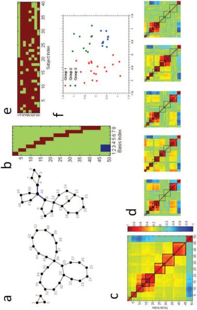
In order to illustrate the behavior of our method, we generated a synthetic dataset with forty instances (or subjects). Our network design is illustrated in Figure 2. Each subject is associated with a fixed underlying network configuration consisting of fifty nodes, as shown in Figure 2a. The “ground truth” SCP basis Btrue is shown in Figure 2b. The network is designed in such a way that it has eight SCPs, with SCP size varying between three-ten nodes. Some of these SCPs are overlapping, with overlap size varying between one-three nodes. The strength of each SCP varies across subjects in a binary fashion, i.e, in each subject, networks are either “active/on” or “inactive/o ”, as shown by the subject-specific coeffcients in Figure 2e. In other words, an SCP is inactive in a subject when all the edges/correlation strengths of that SCP are zero for that particular subject. Furthermore, subjects are categorized into three groups, simulating heterogeneity in subject space. This is shown in Figure 2f, showing the projection of the eight-dimensional coeffcients in 2-D, computed using multi-dimensional scaling (Kruskal, 1964).
Figure 2.
Simulated network design consisting of 50 nodes. (a) Network configuration common to all subjects. Edges in blue indicate anti-correlation. (b) Ground-truth SCP basis Btrue. (c) Subject-averaged correlation matrix. (d) Correlation matrices of five randomly chosen subjects. (e) Subject-specific coefficients for all 40 subjects. (f) Heterogeneity in subject space, shown by the eight-dimensional coefficients projected down to 2-D.
We input this network design into the simulation software NetSim (Smith et al., 2011), which simulates BOLD time-series at each node. Each time-series has 120 time-points and a TR value of 3 seconds (making each dataset 6 minutes long). In addition to inter-subject variability introduced by differential activation of networks we also include small random perturbation of edge strength for all edges. Random external inputs are input to some of the nodes. Thermal (white) noise is added to the output time-series at each node.
Correlation matrices are computed from the simulated time-series for all forty subjects, which form the input to our method. The subject-average correlation matrix is shown in Figure 2c. The matrices shown in Figure 2d correspond to the correlation values computed from the time-series for five randomly chosen subjects.
3.2. Evaluation of results for simulated data
In order to quantify the performance of the algorithm on simulated data, we compare the set of SCPs output by Sparse Learning B with the ground truth Btrue. Before the comparison we first perform a one-to-one matching between the two sets of vectors using the Hungarian Algorithm (Munkres, 1957). The sign of some of the vectors in B is reversed, if necessary. We use the normalized inner product (cosine of the angle between vectors) to compare these paired set of vectors.
We compared the SCPs obtained using Sparse Learning to sub-graphs produced using Infomap (Rosvall and Bergstrom, 2008; Power et al., 2011), TFMs generated using Temporal ICA (Hyvarinen, 1999; Smith et al., 2012) and Intrinsic Connectivity Networks (ICNs) computed using Spatial ICA (Calhoun et al., 2003). The subject-average correlation matrix, thresholded to obtain varying levels of edge density was used as input to InfoMap. Absolute values of correlation were used as input to InfoMap. The clustering assignments output by InfoMap are converted into a set of binary basis vectors, one for each sub-graph. Concatenated time-series data were used as input for Temporal ICA as well as Spatial ICA. In case of ICA, dimensionality reduction was performed by running PCA first, as is routinely done in fMRI-ICA literature (Smith et al., 2012). As before, we used normalized inner product for comparisons with the ground truth.
3.3. Results from simulated data
The output of the cross-validation experiments are shown in the plots in Figures 3, which shows the variation of the cross-validated mean square error as the free parameters, K and λ, are varied. It is clear that the MSE saturates beyond λ = 0.2. Choice of K is somewhat unclear. Using K = 8, λ = 0.2 as the operating point, we computed the basis vectors for the simulated data using all four methods. (Note: For the sampling of edge-densities used to compute results for InfoMap, we were able to obtain K = 7 communities followed by K = 9. As K = 7 has greater accuracy, we display those results.)
Figure 3.
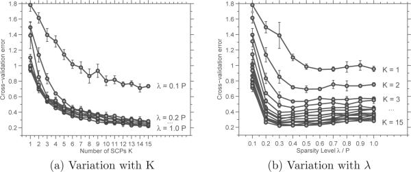
Cross-validation results for simulated data: Plots of the mean square error (Eqn. 3) vs. number of SCPs k (left), and sparsity level λ (right).
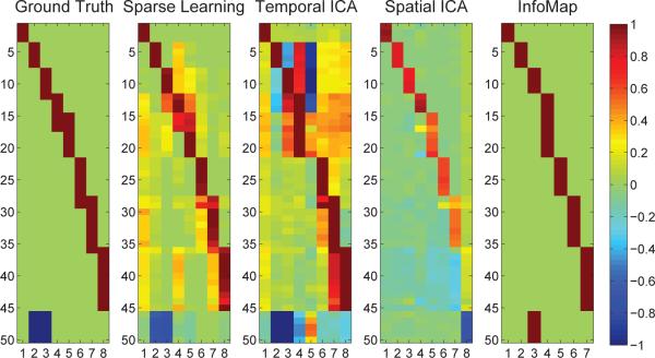
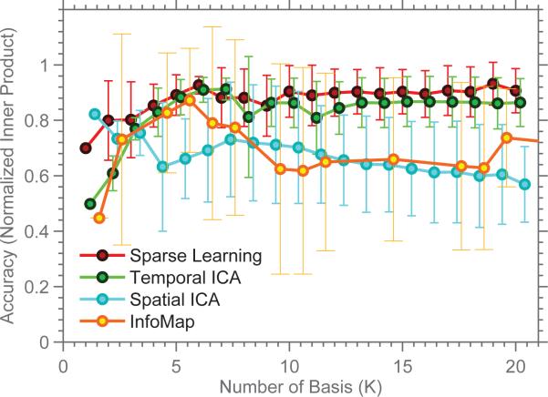
The first image in Figure 4 shows the simulated ground-truth as a vector of node-weights. The results from the four methods are shown next to the ground-truth. Each column displays a basis vector bk. It is easy to see that SCPs computed using Sparse Learning are closest to the ground-truth. We quantify these comparisons with the normalized inner-product measure. Figure 5 shows the accuracy of SCPs, sub-graphs, ICNs and TFMs for varying K. When compared with the ground-truth, SCPs show slightly higher accuracy than the three other methods, for all values of K (p< 0.05, compared at K=8, using a two-sided t-test for Sparse Learning vs. all other methods). Temporal ICA comes a close second, as it is able to capture many of the positive/negative correlations (some false negatives - TFM 5) but results in a denser basis (many false positives). Both Spatial ICA and InfoMap produce non-overlapping ICNs/sub-graphs - and as the value of K is increased, these components get smaller/more fragmented, leading to a drop in accuracy, as seen in the graph.
Figure 4.
Results from simulated data. The basis vectors identified by the sparse learning approach, InfoMap, Spatial and Temporal ICA, shown as node-weights, compared against the ground-truth.
Figure 5.
Accuracy of the results, measured using normalized inner-product.
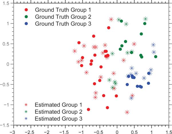
Finally, Figure 6 displays the subject-specific coeffcients estimated by Sparse Learning, along with the ground truth. This result shows that Sparse Learning is able to capture the heterogeneity in the subject-space, since the clustering of the three groups is retained to a large extent in the estimation.
Figure 6.
Subject-specific coeffcients estimated by Sparse Learning, projected down to 2-D space, shown along with the ground truth.
4. Experiments on resting state fMRI data
Having shown that Sparse Learning performs better on synthetic data, we next compared performance of the three methods using resting state data from 130 healthy, young adults between the ages 19 to 22 years, acquired as a part of the Philadelphia Neuro-developmental Cohort (PNC) (Satterthwaite et al., 2014), as detailed below.
4.1. Data
4.1.1. Participants
Resting-state functional connectivity MRI data used here was drawn from the Philadelphia Neuro-developmental Cohort (Satterthwaite et al., 2014), a collaboration between the Center for Applied Genomics at Children's Hospital of Philadelphia (CHOP) and the Brain Behavior Laboratory at the University of Pennsylvania (Penn). Study procedures and design are described elsewhere in detail (Satterthwaite et al., 2014) . Here, in order to minimize the impact of known developmental changes in functional connectivity in this sample (Satterthwaite et al., 2013), we only included subjects greater than 18 years old. Additionally, subjects were excluded if they were being treated with psychotropic medications, had history of inpatient psychiatric treatment, or had a history of medical problems that could potentially impact brain function. We and others have previously demonstrated that motion artifact has a marked confounding influence on resting-state functional connectivity data (Satterthwaite et al., 2013; Power et al., 2011). Accordingly, as in our prior work (Satterthwaite et al., 2013), subjects with a mean relative displacement > 0.2mm (as estimated by FSL's MCFLIRT routine, see below) were excluded from analysis. These inclusion and exclusion criteria resulted in a final sample of 130 subjects, mean age =20.17 (SD=0.79) years, n=58 male. All procedures were approved by the Institutional Review Boards of both Penn and CHOP.
4.1.2. Data acquisition
As described elsewhere in detail (Satterthwaite et al., 2014), all data were acquired on the same scanner (Siemens Tim Trio 3 Tesla, Erlangen, Germany; 32 channel head coil) using the same imaging sequences. Blood oxygen level dependent (BOLD) fMRI was acquired using a whole-brain, single-shot, multi-slice, gradient-echo (GE) echoplanar (EPI) sequence with the following parameters: 124 volumes, TR=3000 ms, TE=32 ms, flip angle=90deg, FOV=192x192 mm, matrix=64X64, slice thickness/gap=3mm/0mm, effective voxel resolution=3.0 x3.0 x3.0mm. Prior to functional time-series acquisition, a magnetization-prepared, rapid acquisition gradient-echo (MPRAGE) T1-weighted image was acquired to aid spatial normalization to standard atlas space, using the following parameters: TR=1810 ms, TE=3.51 ms, FOV=180x240 mm, matrix=256x192, 160 slices, TI=1100 ms, flip angle=9deg, effective voxel resolution of 0.9 x 0.9 x 1mm. During the resting-state scan, a fixation cross was displayed as images were acquired. Subjects were instructed to stay awake, keep their eyes open, fixate on the displayed cross-hair, and remain still.
4.1.3. Node definition
A crucial aspect of functional network estimation is node definition. The high spatial dimensionality of fMRI data makes voxel-wise correlation matrices computationally infeasible for many approaches, hence most studies resort to dimensionality reduction, often through the use of anatomic atlases or through functional parcellation schemes. Nodes based on anatomic definitions often cross functional boundaries, leading to inaccurate network estimation (Smith et al., 2011). Accordingly, as previously (Satterthwaite et al., 2013) we used the 264 nodes defined in Power et al. (2011) (“areal graph”) for our experiments. This network includes 34,716 unique edges. These nodes were defined exclusively based on fMRI. Of these nodes, 151 were non-overlapping 10mm diameter spheres identified based on a meta-analysis of task-fMRI based studies (Dosenbach et al., 2006). The remaining 193 were cortical patches obtained by functional connectivity mapping using resting state fMRI (Cohen et al., 2008). Based on the discrete clustering algorithm Infomap (Rosvall and Bergstrom, 2008), each ROI was categorized by Power et al. (2011) as belonging to one of thirteen non-overlapping sub-graphs.
4.1.4. Registration
Subject-level BOLD images were co-registered to the T1 image using boundary-based registration (Greve and Fischl, 2009) with integrated distortion correction as implemented in FSL 5 (Jenkinson et al., 2012). Whole-head T1 images were registered to the Montreal Neurologic Institute 152 1mm template using the diffeomorphic SyN registration that is part of ANTS (Avants et al., 2008, 2011; Klein et al., 2009). All registrations were inspected manually and also evaluated for accuracy using spatial correlations. Nodes were registered to subject space for timeseries extraction by concatenating the co-registration, distortion correction, and normalization transformations so that only one interpolation was performed in the entire process.
4.1.5. Data processing
A voxel-averaged timeseries was extracted from each of the 264 nodes for every subject. In order to evaluate the impact of motion, data was preprocessed using a validated confound regression procedure that has been optimized to reduce the influence of subject motion (Satterthwaite et al., 2012). The first 4 volumes of the functional timeseries were removed to allow signal stabilization, leaving 120 volumes for subsequent analysis. Functional images were slice-time corrected using slice-timer and re-aligned using MCFLIRT (Jenkinson et al., 2002). Structural images were skull-stripped using BET (Smith, 2002) and segmented using FAST (Zhang et al., 2001); mean white matter (WM) and cerebro-spinal fluid (CSF) signals were extracted from the tissue segments generated for each subject. Confound regression (Satterth-waite et al., 2012) included these 6 standard motion parameters, the WM signal, the CSF signal, and the global signal (i.e., 9 parameters total), as well as the temporal derivative, quadratic term, and temporal derivative of the quadratic of each (36 regressors total). Notably, in order to a avoid a mismatch in the frequency domain (Hallquist et al., 2013), both the confound matrix and the time-series data was simultaneously band-pass filtered to retain signals between 0.01-0.08 Hz using AFNI's 3dBandpass utility (Cox, 1996). Finally, a symmetric connectivity matrix (264x264) was defined for each subject using pairwise Pearson's correlations. This data formed the input to subsequent analyses of functional network structure.
4.2. Evaluation of results for rsfMRI data
4.2.1. Reproducibility
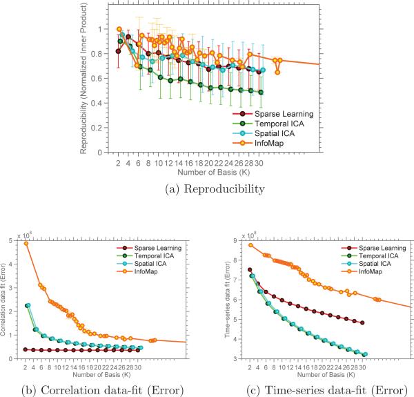
We evaluate the performance of our algorithm as well as Infomap and ICA based on repeated split-sample reproducibility. Reproducibility was evaluated for K = 2, 4, . . . , 30. In the case of InfoMap, the edge-density was varied between 2% and 40%. This provided sub-graphs varying in number from 4 upto 60, although not equally spaced. Similar to our earlier experiments involving simulated data, we quantify the comparison between sub-samples using the normalized inner product, averaged across basis vectors.
4.2.2. Data fit
In addition to reproducibility, the data fit (approximation error) of all the methods to the data was also compared. Given that Sparse Learning and InfoMap use correlation values as input, and ICA methods use time-series as input, we evaluated the approximation error for both types of input. Let B denote the set of basis vectors output by any of the four methods. Let Yn ∈ RP×T and Xn ∈ RK×T be the subject-specific time-series and basis-specific time-series respectively. In the case of Sparse Learning and InfoMap, the basis-specific time-series Xn can be computed by regressing the basis B against the subject-specific time-series Yn. Using these values, the correlation data-fit measure is computed as follows:
| (4) |
where
| (5) |
Similarly the time-series data fit for all four methods is defined as
| (6) |
The correlation data-fit measure is the same as the objective function that is optimized in the Sparse Learning method. Obviously, Sparse Learning is expected to have the best correlation data-fit (lowest error). Similarly, as the ICA methods operate on the time-series as input, they are likely to outperform Sparse Learning and InfoMap with respect to time-series data fit. It is more interesting to note how the correlation methods compare with respect to time-series data fit, and vice versa.
4.2.3. Spatial Overlap and Temporal Correlation
Finally, to further understand the behavior of the methods under consideration, we computed the degree to which the estimated basis vectors are spatially overlapping and temporally correlated. These values are computed as follows:
| (7) |
| (8) |
where xni denotes the time-series associated with the ith basis in the nth subject.
4.2.4. Reproducibility across datasets
To further evaluate the reproducibility of the presented results, we used three publicly available datasets - (1) pilot acquisition dataset from the Human Connectome Project (HCP) (Smith et al., 2012), which has 42 scans acquired at TR = 0.8s, (2) BrainScape Resting State fMRI Dataset 1 (Fox et al., 2007) from the functional Biomedical Informatics Research Network (fBIRN), which has 60 scans acquired at TR = 2s, (3) BrainScape Resting State fMRI Dataset 2 (Fox et al., 2005) from fBIRN, which has 29 scans acquired at TR = 3s. All the scans (131 in total) were pre-processed using the same pipeline that was used for the PNC dataset, as detailed above. All the algorithms (Proposed, InfoMap and ICA) were also run on this alternate dataset.
4.3. Results from rsfMRI data
Figure 7 plots the variation of the cross-validated error as K and λ is varied. From these figures, it is clear that the MSE saturates around λ = 0.3. However, the “knee” of the graph plotting variation with K is unclear.
Figure 7.
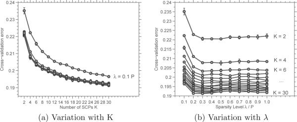
Cross-validation results for PNC data: Plots of the mean square error (Eqn. 3) vs. number of SCPs K (left), and sparsity level λ (right).
Sparse Learning was run on the entire sample of 130 subjects with the values K = 10, λ = 0.3. These ten SCPs are shown in Figures 8, 9, 10 and 11. We describe them in detail below, and compare to existing knowledge of the spatial extent and behavior of known task-processing, attention and control systems.
Figure 8.
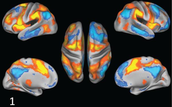
Sparse learning identified a primary Dorsal Attention (DA) SCP, highlighting the anti-correlation between DA and Default Mode (DM)
Figure 9.
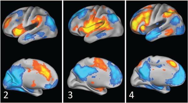
Task-Positive SCPs: SCP 2, 3 and 4 show different regions of the default mode anti-correlated with the Salience, Cingulo-Opercular and Fronto-Parietal control systems respectively.
Figure 10.
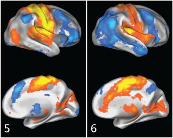
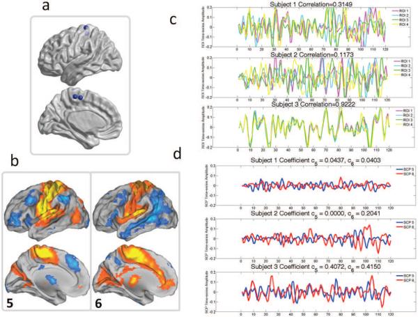
SCPs 5 and 6 show two types of connectivity patterns involving the sensori-motor areas.
Figure 11.
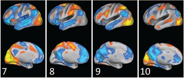
Visual SCPs identified by sparse learning.
Dorsal Attention SCP Figure 8 shows the first SCP defined by the anterior middle temporal area (aMT), superior parietal lobule (SPL), intra parietal sulcus (IPS) and the frontal eye fields (FEF)(shown in red), which are known to be part of the Dorsal Attention (DA) system (Corbetta and Shulman, 2002). These regions are anti-correlated with the middle temporal gyrus (MTG), inferior parietal lobule (IPL), medial pre-frontal cortex(mPFC), posterior cingulate cortex (PCC) and anterior frontal operculum, which are part of the default-mode (DM) system (Raichle et al., 2001)(shown in blue).
Executive Control SCPs Figure 9 displays SCPs 2, 3 and 4 which predominantly show executive task-control system (red) anti-correlated with different aspects of the DM system (blue). SCP 4 shows the Salience system (Seeley et al., 2007) consisting of dorsal anterior cingulate cortex (dACC) along with anterior insula and the anterior pre-frontal cortex. The anti-correlated DM regions include the IPL, PCC and vmPFC. Regions from the operculum, insula, temporal-parietal junction (TPJ), inferior frontal gyrus (IFG) and the dACC dominate SCP 5, with anti-correlations to PCC and dmPFC. This SCP consists of the Cingulo-Opercular (COP) system (Dosen-bach et al., 2007) which is known to de-activate the DM. SCP 6 consists of the aPFC, aI, IPL, and MT, which form the Fronto Parietal task-control system, anti-correlating with the inferior MTG, IPL, PCC, mPFC and PHC.
Motor SCPs Figure 10 shows SCPs 5 and 6, which exhibit contributions from the sensori-motor, auditory and visual areas. Both SCPs show the pre central (prCG) and post central gyrus (poCG). In SCP 5 the motor areas positively correlate with the superior temporal gyrus (STG) and posterior insula. The positive correlations in SCP 6 are more anterior within the insula, and a large extent of the cingulum. Anti-correlated regions include the FP system (aPFC, IPL, aI, ACC) in SCP 5 and aspects of the DM system in SCP 6.
Visual SCPs SCPs 7, 8, 9 and 10 in Figure 11 show four types of connectivity patterns involving the visual areas. SCP 7 covers the entire visual system, including the medial visual, lateral visual and higher visual (dorsal attention) areas. SCP 8 shows the higher visual areas alone. The visual areas are anti-correlated with the DM system in both the SCPs. SCPs 9 and 10 shows contributions from areas in the lower levels of the visual hierarchy; the FEF and the prCS are less dominant, while including the lateral visual areas, which are involved in higher level visual task-processing. Concomitant with moving down along the hierarchy, we observe changes to the anti-correlated regions - the involvement of the mPFC is greatly reduced, but the anti-correlation the posterior cingulate is retained.
Overlap between SCPs The SCPs described above are clearly overlapping, mainly enabling the description of multiple relationships between a functional system and other systems. We note that the PCC and the IPL contribute to most of the SCPs, which were identified by a prior study as one of the central hubs of connectivity in the brain (Buckner et al., 2009).
Inter-subject variability Differential presence of the SCPs explains inter subject variability in functional connectivity. Figure 12 shows the strength of presence of each SCP in every subject. The Sparse Learning approach exploits this variability; a heterogeneous distribution of the samples in this lower-dimensional space allows robust identification of the SCPs.
Figure 12.

Figure illustrating the heterogeneity of the data sample captured by SCPs. The color indicates the extent to which each SCP is present in a subject.
A simple case illustrating the manner in which Sparse Learning captures inter-subject variability is shown Figure 13. We considered four ROIs within the sensori-motor areas (shown in Figure 13a). These four ROIs participate in SCP 5 as well as SCP 6, as seen in Figure 13b. The corresponding time-series for the four ROIs are shown in Figure 13c, for three subjects, which have varying amounts of correlation between them. In the first two subjects, the time-series observed at these four ROIs are asynchronous, making their average pair-wise correlation low (0.32 and 0.12 respectively). This has two consequences. Firstly, this inter-subject variability is reflected in the SCP coeffcients; for the first subject, both c5 and c6 are low, and for the second subject c5 is zero. Similarly, (almost) perfect synchronization among these four time-series is reflected in the higher values assigned to both c5 and c6. Secondly, this also affects the SCP time-series that are computed after the SCP vectors B are found. Low correlation between the ROIs leads to SCP time-series with very low amplitude, as seen in the first subject.
Figure 13.
Inter-subject variability in SCP coeffcients, and their associated time-courses. (a) Location of the four ROIs (b) SCP 5 and 6, that the four ROIs are associated with (c) Time-series at each of the four ROIs in three different subjects (d) The coeffcients c5 and c6 of the three subjects, along with the associated SCP time-courses
4.3.1. Reproducibility and Approximation error
Recall that in order to test the generalizability of our results, we ran repeated split-sample validation, comparing the results using normalized inner-product. The reproducibility of the results is shown in Figure 14a, computed for values of K ∈ 2, 4, . . . , 30. For K = 10, the reproducibility of our results is 0.80 ± 0.09, compared to 0.86 ± 0.15 for InfoMap, 0.79 ± 0.07 for Spatial ICA and 0.60 ± 0.12 for Temporal ICA. InfoMap shows comparable reproducibility with sparse learning (p < 0.4, computed using two-group t-test). Spatial ICA components are as reproducible as Sparse Learning (p < 0.8), while Temporal ICA performs significantly worse (p < 10−4) in terms of reproducibility. Figure 14b and 14c show the correlation data-fit and the time-series data-fit of all the methods for varying values of K. InfoMap performs poorly in terms of data-fit for both correlation as well as time-series data. As expected, Sparse Learning has the best correlation data-fit, while the ICA methods provide the best time-series data fit.
Figure 14.
Reproducibility and data-fit measured for SCPs obtained from rsfMRI dataset.
4.3.2. Spatial Overlap and Temporal Correlation
As expected, InfoMap has no spatial overlap in its basis. Spatial ICA shows decreasing overlap with increasing K, as shown in Figure 15a. Sparse Learning has the highest spatial overlap. Figure 15b shows the variation of the average temporal correlation with K. Temporal ICA has no temporal correlation while Spatial ICA has the highest temporal correlation. Of the four methods, only Sparse Learning has non zero spatial overlap as well as temporal correlation.
Figure 15.
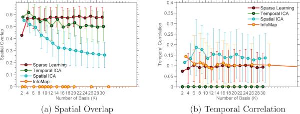
Spatial overlap and Temporal correlation measured for SCPs obtained from rsfMRI dataset.
4.3.3. Reproducibility across datasets
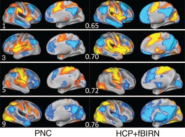
To further evaluate the reproducibility of the presented results, we compared them with SCPs computed from the alternate HCP+fBIRN dataset. We found that the SCPs are reasonably reproduced in the alternate dataset, with an average inner-product 0.65 ± 0.07. A side-by-side comparison of four SCPs computed from the PNC and alternate datasets is shown in Figure 16.
Figure 16.
SCPs 1, 2, 5, and 9 computed from the PNC dataset(left) and HCP/fBIRN dataset (right). The inner product value for each comparison is also shown.
4.3.4. Comparison with sub-graphs and TFMs
InfoMap assigned major functional systems to different sub-graphs. This is consistent with findings reported in Power et al. (2011). The task-positive regions are assigned to separate sub-graphs (sub-graphs 4, 5 and 7 shown in SI Figure 1). All task-negative default-mode regions form a single entity (sub-graph 2). Sparse Learning also assigns task-positive regions to separate SCPs, but in addition also reveals regions belonging to the DM system that are negatively coupled with them. The sensory areas are assigned to two separate sub graphs, visual and motor (sub graphs 1 and 3), while SCPs 9 and 10 uncover the manner in which they can correlate. The behavior of PCC and IPL regions as cortical “hubs” (Buckner et al., 2009), cannot be surmised from the sub-graphs found using InfoMap.
On the other hand, TFMs identified using ICA are spatially overlapping and incorporate negative values. Of the ten, two SCPs 1 and 8 can also be found using ICA (SI Figure 2). The rest are in general quite different from the results seen here. Unlike sub-graphs and SCPs, ICA is unable to clearly separate task-positive systems into different components, due to possible temporal co-activation of these systems.
5. Discussion
The findings presented in this paper are obtained from a connectivity-based modeling approach that identifies SCPs based on important observations - (1) Not all brain regions participate in a given SCP; (2) regions that belong to an SCP are functionally coherent, or correlated (or anti-correlated); and (3) if a set of regions act as an SCP, then, in a set of normal subjects, inter-subject variability is introduced due to the different extent to which each SCP is active in a subject. Sparse Learning is able to separate task-positive regions and their associated task-negative regions into separate SCPs in a data-driven manner, without requiring a-priori knowledge of a “seed” region. Sparse Learning is able to provide additional insights by allowing for spatial overlap between SCPs as well as positive and negative correlations within the same SCP. These features of the approach make it possible to assign overlapping subsets of regions within a functional system to different SCPs, facilitating a description of their varied relationships with other regions of the brain.
5.1. Observations based on simulated experiments
Based on the simulated ground truth experiments, compared to Sparse Learning, both InfoMap and ICA are also able to capture many of the correlated/anti-correlated relationships between regions. However, as the simulation results show, their inherent methodological constraints result in networks with lower accuracy (for InfoMap and Spatial ICA). InfoMap and Spatial ICA are able to identify strongly correlated sets of nodes, while avoiding the points of overlap. The spatial segregation constraint causes a region that belongs to multiple networks to get assigned to a single network, possibly the one with which it has the strongest correlation. Similarly, Temporal ICA is able to reveal the true relationship between nodes to some extent. For example, within basis vectors 2-4 (Figure 4), while it is able to reveal the positive correlation between the nodes, it also requires participation from the other nodes, in order to be able to maximally unmix the data into independent temporal components (they are temporally dependent by design; there are some instances (subjects) where SCP 2 co-activates with the other SCPs, making them dependent). If multiple spatially overlapping networks activate together in some subjects, resulting in a moderate amount of temporal correlation between them, ICA assigns all these networks to the same TFM ( as it tries to maximize independence between TFMs). In contrast, if these multiple networks show differential strengths in subjects, even though they are spatially and temporally dependent, the Sparse Learning approach can separate them into different SCPs.
The results shown in Figure 4 also illustrate a potential limitation of the proposed method; when the network sizes are unbalanced, such as in the simulation design used here, using the same sparsity level λ is inappropriate. Picking a value of λ less than size of the largest SCP leads to those SCP getting truncated, and is sub-optimal. On the other hand, picking a value equal to the size of the largest community (= 20% in the simulated case) leads to noisy assignments in the smallest community, i.e, SCP 1, as seen in Figure 4. This limitation is similar to that of the edge density parameter used in InfoMap, where lower edge density leads to smaller communities. In practice, however, these false (noisy) assignments that are incorporated in the basis are generally very weak (have low absolute values).
The ability to quantify the strength of presence of an SCP at the level of individual subjects provides us with a framework for population studies, as illustrated by the simulated data in Figure 6. This advantage cannot be found in seed-based correlation methods or graph-partitioning approaches. Although we did not perform subject-specific analyses, the sparse decomposition framework adopted herein is a powerful tool for exploring such population heterogeneities in the future, and potentially leading to diagnostic and predictive functional connectivity biomarkers. SCP coefficient values ci are comparable across subjects within the same SCP. Univariate SCP-wise analyses can be performed to look for differences relative to known/latent subgroups. Similarly, multi-variate analyses that consider all the coeffcients ci of a subject i as a feature vector can lead to potentially insightful results.
5.2. Interpretation of rsfMRI SCP findings
As the results from rsfMRI data (Figures 8,9,10,11) show, this approach is able to separate task-positive regions and their associated task-negative regions into separate SCPs in a data-driven manner, without requiring knowledge of a “seed” region of interest. SCP 1 in Figure 8 shows anti-correlation between the Dorsal Attention system and the Default Mode. This anti-correlation is a well-known finding (Fox et al., 2005), found using seed-based correlation. In Figure 9, we see the task-positive systems - Cingulo Opercular, Salience and Fronto-Parietal task control. As seen in the patterns, all are known to deactivate the default mode system. This was described first using seed-based correlation (Seeley et al., 2007; Dosenbach et al., 2007), and more recently demonstrated using non-invasive brain stimulation (Chen et al., 2013). Of greater interest is the differential contribution of regions belonging to the DM within these SCPs (regions in blue). PCC shows steady contributions, while the lateral default mode areas are more variable.
SCPs 5-10 relate to the task-processing motor and visual areas, shown in Figures 10 and 11. SCPs 5 and 6 show two connectivity patterns that involve the sensori-motor areas and its anti-correlations. These patterns are reproducible across datasets to some extent (see Figure 16, SCP 5), contrary to an earlier report (Tian et al., 2007). The visual areas display multiple different patterns of connectivity as seen in SCPs 7-10, with either the higher visual (dorsal attention) areas only (SCP 8), lateral visual only (SCP 9) or both lateral and medial visual areas (SCP 7 and 10). All four SCPs show varying amounts of anti-correlation with the default-mode system. Thus, Sparse Learning is able to provide additional insights by allowing for spatial overlap between SCPs as well as positive and negative correlations within the same SCP. These features of the approach make it possible to assign overlapping subsets of regions within a functional system to different SCPs, facilitating a description of their varied relationships with other regions of the brain.
The reproducibility of the SCPs described above is reasonably high, as shown in Figure 14a for comparison within the same dataset, and Figure 16, across datasets. Although the basis obtained using InfoMap and Spatial ICA are reliably reproduced, results from simulated data suggest that these results may not be very accurate, as it comes at the cost of ignoring regions of overlap and anti-correlated relationships, thus trading accuracy for greater reproducibility (Figure 4). This is also reflected in the data-fit plots shown in Figure 14b and 14c, computed using rsfMRI data. Furthermore, of the four methods considered, Sparse Learning is the only method that does not constrain its basis to be spatially or temporally segregated, as seen in Figure 15.
5.3. Related methods, limitations and future work
The Sparse Learning approach used herein finds sparse patterns based on second-order statistics (correlation) in each subject's data. While this may resemble PCA, sparse PCA (sPCA)(Moghaddam et al., 2005; d'Aspremont et al., 2008) and their variant analysis approaches, there are several important differences. PCA and sPCA (Moghaddam et al., 2005; d'Aspremont et al., 2008) find directions of maximum variance based on a single covariance matrix common to all data. The proposed method is a matrix factorization problem, in which we consider the correlation matrix corresponding to each subject as an independent observation. This allows us to model inter-subject variability in the correlations by encoding it in the coeffcients cn. Furthermore, in PCA and sPCA the sparse basis vectors are computed in sequence, one after another. After each basis vector is computed, the projection of the data along this basis is removed from the data, using Matrix Deflation (Mackey, 2009). In practice, removing the projection of the data on the kth basis causes the (k + 1)th basis to be mostly unrelated to the kth basis, i.e., the resulting basis vectors are approximately orthogonal. This is not the case with the proposed Sparse Learning algorithm, which simultaneously estimates the basis vectors, with the intent of avoiding orthogonality (See SI Figure 4). Finally, the objective function that is optimized is substantially different between the two approaches. PCA and sPCA maximize the variance along the basis direction bk, which is second-order in the variable bk. The objective function of the proposed method is fourth order in the same variable.
In the rsfMRI literature, correlation is probably the most widely used connectivity measure, with precision measures advocated more recently (Varoquaux et al., 2010). The precision matrix is the inverse of the covariance matrix, and its elements are related to partial correlation. For most standard rsfMRI datasets, the dimensionality of the data is larger than the number of samples (time-points). In such a case additional assumptions are required to be able to invert the correlation matrix, typically either via shrinkage or using sparse prior (Varoquaux et al., 2010). These two measures (correlation and precision) answer somewhat different questions, both useful - precision matrices mitigate indirect connections, attempting to find the “true” underlying connnections (Smith et al., 2011), while correlation is the simplest pair-wise measure, used widely for dimensionality reduction/community detection. We preferred correlation because when the basis B is sparse, the matrix BCBT loosely displays a block-diagonal structure, similar to what we typically observe in correlation matrices. Thus, the proposed method takes advantage of these indirect connections which make up the blocks. Inverting the correlation matrix removes this block-diagonal structure (the dense but indirect connections within the blocks are lost), hence a BCBT type of approximation becomes no longer appropriate for precision matrices.
SCPs presented in this paper were obtained after removing the baseline global signal from each subject's data, which facilitates the delineation of functional systems by removing the confounding e ects of motion and other non-neuronal sources of noise (Fox et al., 2009). On the other hand, many researchers argue that performing Global Signal Regression (GSR) on rsfMRI data removes relevant signal and tends to increase the number of negatively correlated nodes (Saad et al., 2012). It is unclear if the high reproducibility of our results reflects true signal, or a systematic artifact induced due to global signal regression. Hence we re-ran Sparse Learning with the global signal retained. SCPs continued to be reproducible, however they were substantively different. Of the ten SCPs computed, only one SCP had a significant areas of negative correlation - the Dorsal Attention vs. Default mode anti-correlation pattern. The other nine SCPs showed only positive correlations. Of these, the familiar SCP patterns were the sensori-motor, visual and cingulo-opercular networks (see SI Figure 3).
Note that in the current implementation we use random values to initialize the variables. We found that repeated random initializations gave very similar results. However, we this might not always be the case. Low sample sizes, high dimensionality of the data and large values of K will have a large impact on the stability of the results. Keeping this in mind, in future implementations we will use multiple starting values and pick SCPs that recur across runs.
The proposed method is a versatile framework that can be combined with other modules to obtain specific SCPs that can explain variation along a certain dimension. For example in our preliminary work in Eavani et al. (2013), we used sparse learning within a state-space model to identify modes of temporal variation, or “brain-states”, which has been the focus of many studies in recent years (Chang and Glover, 2010; Leonardi et al., 2013; Janoos et al., 2013). This framework can also be combined with a discriminative term (Batmanghelich et al., 2012; Eavani et al., 2014) to obtain functional bio-markers for disease.
6. Conclusions
In this paper, we used recent advances in the mathematics of sparse modeling to obtain a parsimonious representation of brain function. The presented findings o er novel insights into the organization of brain function and effectively captures the heterogeneity of functional organization across individuals. These results are reliably reproduced between sub-samples of data as well as across datasets, and advance existing knowledge of intrinsic connectivity patterns. The novelty and reproducibility of our results across datasets make a compelling argument for the usage of sparse representations to model fMRI connectivity. These results, taken together with those from other approaches, provide a more complete picture that can help elucidate the functional organization of the brain.
Supplementary Material
Highlights.
- Sparse, low rank decomposition for the analysis of functional connectivity matrices
- Resulting Sparse Connectivity Patterns (SCPs) include both pos and neg correlations
- SCPs are not restricted to be orthogonal or independent
- SCPs are reliably reproduced between split-samples as well as in replication dataset
- Resulting SCP coeffs show inter-subject variation, a useful measure for group studies
Acknowledgements
The authors would like to thank Stephen Smith and Mark Woolrich for providing the code for the NetSim simulation software (Smith et al., 2011). This work was partially supported by NIH grant AG014971, NIMH grants MH089983 and MH089924, as well as T32 MH019112. Dr. Satterthwaite was supported by K23MH098130 and the Marc Rapport Family Investigator grant through the Brain and Behavior Foundation. We would also like to thank our anonymous reviewers whose helpful suggestions have greatly improved this manuscript.
Footnotes
Publisher's Disclaimer: This is a PDF file of an unedited manuscript that has been accepted for publication. As a service to our customers we are providing this early version of the manuscript. The manuscript will undergo copyediting, typesetting, and review of the resulting proof before it is published in its final citable form. Please note that during the production process errors may be discovered which could affect the content, and all legal disclaimers that apply to the journal pertain.
References
- Ahn YY, Bagrow JP, Lehmann S. Link communities reveal multiscale complexity in networks. Nature. 2010;466:761–764. doi: 10.1038/nature09182. [DOI] [PubMed] [Google Scholar]
- Avants BB, Epstein CL, Grossman M, Gee JC. Symmetric di eomorphic image registration with cross-correlation: evaluating automated labeling of elderly and neurodegenerative brain. Medical image analysis. 2008;12:26–41. doi: 10.1016/j.media.2007.06.004. [DOI] [PMC free article] [PubMed] [Google Scholar]
- Avants BB, Tustison NJ, Song G, Cook PA, Klein A, Gee JC. A reproducible evaluation of ants similarity metric performance in brain image registration. Neuroimage. 2011;54:2033–2044. doi: 10.1016/j.neuroimage.2010.09.025. [DOI] [PMC free article] [PubMed] [Google Scholar]
- Bansal N, Blum A, Chawla S. Correlation clustering. Machine Learning. 2004;56:89–113. [Google Scholar]
- Batmanghelich N, Taskar B, Davatzikos C. Generative-discriminative basis learning for medical imaging. Medical Imaging, IEEE Transactions on. 2012;31:51–69. doi: 10.1109/TMI.2011.2162961. [DOI] [PMC free article] [PubMed] [Google Scholar]
- Biswal B, Zerrin Yetkin F, Haughton VM, Hyde JS. Functional connectivity in the motor cortex of resting human brain using echo-planar mri. Magnetic resonance in medicine. 1995;34:537–541. doi: 10.1002/mrm.1910340409. [DOI] [PubMed] [Google Scholar]
- Buckner RL, Sepulcre J, Talukdar T, Krienen FM, Liu H, Hedden T, Andrews-Hanna JR, Sperling RA, Johnson KA. Cortical hubs revealed by intrinsic functional connectivity: mapping, assessment of stability, and relation to alzheimer's disease. The Journal of Neuroscience. 2009;29:1860–1873. doi: 10.1523/JNEUROSCI.5062-08.2009. [DOI] [PMC free article] [PubMed] [Google Scholar]
- Calhoun V, Adali T, Hansen L, Larsen J, Pekar J. Ica of functional mri data: an overview. in Proceedings of the International Workshop on Independent Component Analysis and Blind Signal Separation; Citeseer. 2003. [Google Scholar]
- Chang C, Glover GH. Time–frequency dynamics of resting-state brain connectivity measured with fmri. Neuroimage. 2010;50:81–98. doi: 10.1016/j.neuroimage.2009.12.011. [DOI] [PMC free article] [PubMed] [Google Scholar]
- Chen AC, Oathes DJ, Chang C, Bradley T, Zhou ZW, Williams LM, Glover GH, Deisseroth K, Etkin A. Causal interactions between fronto-parietal central executive and default-mode networks in humans. Proceedings of the National Academy of Sciences. 2013:201311772. doi: 10.1073/pnas.1311772110. [DOI] [PMC free article] [PubMed] [Google Scholar]
- Cohen AL, Fair DA, Dosenbach NU, Miezin FM, Dierker D, Van Essen DC, Schlaggar BL, Petersen SE. Defining functional areas in individual human brains using resting functional connectivity mri. Neuroimage. 2008;41:45. doi: 10.1016/j.neuroimage.2008.01.066. [DOI] [PMC free article] [PubMed] [Google Scholar]
- Corbetta M, Shulman GL. Control of goal-directed and stimulus-driven attention in the brain. Nature reviews neuroscience. 2002;3:201–215. doi: 10.1038/nrn755. [DOI] [PubMed] [Google Scholar]
- Cox RW. Afni: software for analysis and visualization of functional magnetic resonance neuroimages. Computers and Biomedical research. 1996;29:162–173. doi: 10.1006/cbmr.1996.0014. [DOI] [PubMed] [Google Scholar]
- d'Aspremont A, Bach F, Ghaoui LE. Optimal solutions for sparse principal component analysis. The Journal of Machine Learning Research. 2008;9:1269–1294. [Google Scholar]
- Ding C, He X. Proceedings of the twenty-first international conference on Machine learning. ACM; 2004. K-means clustering via principal component analysis; p. 29. [Google Scholar]
- Ding CH, He X, Simon HD. On the equivalence of nonnegative matrix factorization and spectral clustering. SDM. 2005:606–610. [Google Scholar]
- Dosenbach N, Fair D, Miezin F, Cohen A, et al. Distinct brain networks for adaptive and stable task control in humans. Proceedings of the National Academy of Sciences. 2007;104(26):11073. doi: 10.1073/pnas.0704320104. [DOI] [PMC free article] [PubMed] [Google Scholar]
- Dosenbach NU, Visscher KM, Palmer ED, Miezin FM, Wenger KK, Kang HC, Burgund ED, Grimes AL, Schlaggar BL, Petersen SE, et al. A core system for the implementation of task sets. Neuron. 2006;50:799. doi: 10.1016/j.neuron.2006.04.031. [DOI] [PMC free article] [PubMed] [Google Scholar]
- Eavani H, Satterthwaite TD, Gur RE, Gur RC, Davatzikos C. Information Processing in Medical Imaging. Springer; 2013. Unsupervised learning of functional network dynamics in resting state fmri; pp. 426–437. [DOI] [PMC free article] [PubMed] [Google Scholar]
- Eavani H, Satterthwaite TD, Gur RE, Gur RC, Davatzikos C. Medical Image Computing and Computer-Assisted Intervention–MICCAI 2014. Springer International Publishing; 2014. Discriminative sparse connectivity patterns for classification of fmri data; pp. 193–200. [DOI] [PMC free article] [PubMed] [Google Scholar]
- Fox MD, Corbetta M, Snyder AZ, Vincent JL, Raichle ME. Spontaneous neuronal activity distinguishes human dorsal and ventral attention systems. Proceedings of the National Academy of Sciences. 2006;103:10046–10051. doi: 10.1073/pnas.0604187103. [DOI] [PMC free article] [PubMed] [Google Scholar]
- Fox MD, Snyder AZ, Vincent JL, Corbetta M, Van Essen DC, Raichle ME. The human brain is intrinsically organized into dynamic, anticorrelated functional networks. Proceedings of the National Academy of Sciences of the United States of America. 2005;102:9673–9678. doi: 10.1073/pnas.0504136102. [DOI] [PMC free article] [PubMed] [Google Scholar]
- Fox MD, Snyder AZ, Vincent JL, Raichle ME. Intrinsic fluctuations within cortical systems account for intertrial variability in human behavior. Neuron. 2007;56:171–184. doi: 10.1016/j.neuron.2007.08.023. [DOI] [PubMed] [Google Scholar]
- Fox MD, Zhang D, Snyder AZ, Raichle ME. The global signal and observed anticorrelated resting state brain networks. Journal of neurophysiology. 2009;101:3270–3283. doi: 10.1152/jn.90777.2008. [DOI] [PMC free article] [PubMed] [Google Scholar]
- Greicius MD, Srivastava G, Reiss AL, Menon V. Default-mode network activity distinguishes alzheimer's disease from healthy aging: evidence from functional mri. Proceedings of the National Academy of Sciences of the United States of America. 2004;101:4637–4642. doi: 10.1073/pnas.0308627101. [DOI] [PMC free article] [PubMed] [Google Scholar]
- Greve DN, Fischl B. Accurate and robust brain image alignment using boundary-based registration. Neuroimage. 2009;48:63–72. doi: 10.1016/j.neuroimage.2009.06.060. [DOI] [PMC free article] [PubMed] [Google Scholar]
- von dem Hagen EA, Stoyanova RS, Baron-Cohen S, Calder AJ. Reduced functional connectivity within and between 'social’ resting state networks in autism spectrum conditions. Social cognitive and a ective neuroscience . 2012 doi: 10.1093/scan/nss053. [DOI] [PMC free article] [PubMed] [Google Scholar]
- Hallquist MN, Hwang K, Luna B. The nuisance of nuisance regression: Spectral misspecification in a common approach to resting-state fmri preprocessing reintroduces noise and obscures functional connectivity. NeuroImage . 2013 doi: 10.1016/j.neuroimage.2013.05.116. [DOI] [PMC free article] [PubMed] [Google Scholar]
- He BJ, Snyder AZ, Vincent JL, Epstein A, Shulman GL, Corbetta M. Breakdown of functional connectivity in frontoparietal networks underlies behavioral deficits in spatial neglect. Neuron. 2007;53:905–918. doi: 10.1016/j.neuron.2007.02.013. [DOI] [PubMed] [Google Scholar]
- Hyvarinen A. Fast ica for noisy data using gaussian moments, in: Circuits and Systems, 1999. ISCAS’99. Proceedings of the 1999 IEEE International Symposium on, IEEE. 1999:57–61. [Google Scholar]
- Janoos F, Brown G, Mórocz I, Wells W. State-space analysis of working memory in schizophrenia: An fbirn study. Psychometrika. 2013;78:279–307. doi: 10.1007/s11336-012-9300-6. [DOI] [PMC free article] [PubMed] [Google Scholar]
- Jenkinson M, Bannister P, Brady M, Smith S. Improved optimization for the robust and accurate linear registration and motion correction of brain images. Neuroimage. 2002;17:825–841. doi: 10.1016/s1053-8119(02)91132-8. [DOI] [PubMed] [Google Scholar]
- Jenkinson M, Beckmann CF, Behrens TE, Woolrich MW, Smith SM. Fsl. NeuroImage. 2012;62:782–790. doi: 10.1016/j.neuroimage.2011.09.015. [DOI] [PubMed] [Google Scholar]
- Keller CJ, Bickel S, Honey CJ, Groppe DM, Entz L, Craddock RC, Lado FA, Kelly C, Milham M, Mehta AD. Neurophysiological investigation of spontaneous correlated and anticorrelated fluctuations of the bold signal. The Journal of Neuroscience. 2013;33:6333–6342. doi: 10.1523/JNEUROSCI.4837-12.2013. [DOI] [PMC free article] [PubMed] [Google Scholar]
- Klein A, Andersson J, Ardekani BA, Ashburner J, Avants B, Chiang MC, Christensen GE, Collins DL, Gee J, Hellier P, et al. Evaluation of 14 nonlinear deformation algorithms applied to human brain mri registration. Neuroimage. 2009;46:786–802. doi: 10.1016/j.neuroimage.2008.12.037. [DOI] [PMC free article] [PubMed] [Google Scholar]
- Kruskal JB. Multidimensional scaling by optimizing goodness of fit to a nonmetric hypothesis. Psychometrika. 1964;29:1–27. [Google Scholar]
- Leonardi N, Richiardi J, Gschwind M, Simioni S, Annoni JM, Schluep M, Vuilleumier P, Van De Ville D. Principal components of functional connectivity: A new approach to study dynamic brain connectivity during rest. NeuroImage. 2013;83:937–950. doi: 10.1016/j.neuroimage.2013.07.019. [DOI] [PubMed] [Google Scholar]
- Mackey LW. Deflation methods for sparse pca. Advances in neural information processing systems. 2009:1017–1024. [Google Scholar]
- Mayer AR, Mannell MV, Ling J, Gasparovic C, Yeo RA. Functional connectivity in mild traumatic brain injury. Human brain mapping. 2011;32:1825–1835. doi: 10.1002/hbm.21151. [DOI] [PMC free article] [PubMed] [Google Scholar]
- Moghaddam B, Weiss Y, Avidan S. Spectral bounds for sparse pca: Exact and greedy algorithms. Advances in neural information processing systems. 2005:915–922. [Google Scholar]
- Munkres J. Algorithms for the assignment and transportation problems. Journal of the Society for Industrial & Applied Mathematics. 1957;5:32–38. [Google Scholar]
- Newman ME. Fast algorithm for detecting community structure in networks. Physical review E. 2004;69:066133. doi: 10.1103/PhysRevE.69.066133. [DOI] [PubMed] [Google Scholar]
- Ng B, McKeown MJ, Abugharbieh R. Group replicator dynamics: A novel group-wise evolutionary approach for sparse brain network detection. Medical Imaging, IEEE Transactions on. 2012;31:576–585. doi: 10.1109/TMI.2011.2173699. [DOI] [PubMed] [Google Scholar]
- Power JD, Cohen AL, Nelson SM, Wig GS, Barnes KA, Church JA, Vogel AC, Laumann TO, Miezin FM, Schlaggar BL, Petersen SE. Functional network organization of the human brain. Neuron. 2011;72:665–678. doi: 10.1016/j.neuron.2011.09.006. doi:10.1016/j.neuron.2011.09.006. [DOI] [PMC free article] [PubMed] [Google Scholar]
- Raichle M, MacLeod A, Snyder A, Powers W, Gusnard D, Shulman G. A default mode of brain function. Proceedings of the National Academy of Sciences. 2001;98:676–682. doi: 10.1073/pnas.98.2.676. [DOI] [PMC free article] [PubMed] [Google Scholar]
- Rosvall M, Bergstrom CT. Maps of random walks on complex networks reveal community structure. Proceedings of the National Academy of Sciences. 2008;105:1118–1123. doi: 10.1073/pnas.0706851105. [DOI] [PMC free article] [PubMed] [Google Scholar]
- Rubinov M, Sporns O. Weight-conserving characterization of complex functional brain networks. Neuroimage. 2011;56:2068–2079. doi: 10.1016/j.neuroimage.2011.03.069. [DOI] [PubMed] [Google Scholar]
- Saad ZS, Gotts SJ, Murphy K, Chen G, Jo HJ, Martin A, Cox RW. Trouble at rest: how correlation patterns and group di erences become distorted after global signal regression. Brain connectivity. 2012;2:25–32. doi: 10.1089/brain.2012.0080. [DOI] [PMC free article] [PubMed] [Google Scholar]
- Satterthwaite TD, Elliott MA, Gerraty RT, Ruparel K, Loughead J, Calkins ME, Eickho SB, Hakonarson H, Gur RC, Gur RE, et al. An improved framework for confound regression and filtering for control of motion artifact in the preprocessing of resting-state functional connectivity data. Neuroimage . 2012 doi: 10.1016/j.neuroimage.2012.08.052. [DOI] [PMC free article] [PubMed] [Google Scholar]
- Satterthwaite TD, Elliott MA, Ruparel K, Loughead J, Prabhakaran K, Calkins ME, Hopson R, Jackson C, Keefe J, Riley M, et al. Neuroimaging of the philadelphia neurodevelopmental cohort. NeuroImage. 2014;86:544–553. doi: 10.1016/j.neuroimage.2013.07.064. [DOI] [PMC free article] [PubMed] [Google Scholar]
- Satterthwaite TD, Wolf DH, Loughead J, Ruparel K, Valdez JN, Siegel SJ, Kohler CG, Gur RE, Gur RC. Association of enhanced limbic response to threat with decreased cortical facial recognition memory response in schizophrenia. American Journal of Psychiatry. 2010;167:418–426. doi: 10.1176/appi.ajp.2009.09060808. [DOI] [PMC free article] [PubMed] [Google Scholar]
- Satterthwaite TD, Wolf DH, Ruparel K, Erus G, Elliott MA, Eickho SB, Gennatas ED, Jackson C, Prabhakaran K, Smith A, et al. Heterogeneous impact of motion on fundamental patterns of developmental changes in functional connectivity during youth. NeuroImage. 2013;83:45–57. doi: 10.1016/j.neuroimage.2013.06.045. [DOI] [PMC free article] [PubMed] [Google Scholar]
- Seeley WW, Menon V, Schatzberg AF, Keller J, Glover GH, Kenna H, Reiss AL, Greicius MD. Dissociable intrinsic connectivity networks for salience processing and executive control. The Journal of neuroscience. 2007;27:2349–2356. doi: 10.1523/JNEUROSCI.5587-06.2007. [DOI] [PMC free article] [PubMed] [Google Scholar]
- Sivalingam R, Boley D, Morellas V, Papanikolopoulos N. Positive definite dictionary learning for region covariances. Computer Vision (ICCV), 2011 IEEE International Conference on, IEEE. 2011:1013–1019. [Google Scholar]
- Smith S, Miller K, Moeller S, Xu J, Auerbach E, Woolrich M, Beckmann C, Jenkinson M, Andersson J, Glasser M, et al. Temporally-independent functional modes of spontaneous brain activity. Proceedings of the National Academy of Sciences. 2012;109:3131–3136. doi: 10.1073/pnas.1121329109. [DOI] [PMC free article] [PubMed] [Google Scholar]
- Smith SM. Fast robust automated brain extraction. Human brain mapping. 2002;17:143–155. doi: 10.1002/hbm.10062. [DOI] [PMC free article] [PubMed] [Google Scholar]
- Smith SM, Miller KL, Salimi-Khorshidi G, Webster M, Beckmann CF, Nichols TE, Ramsey JD, Woolrich MW. Network modelling methods for fmri. Neuroimage. 2011;54:875–891. doi: 10.1016/j.neuroimage.2010.08.063. [DOI] [PubMed] [Google Scholar]
- Sra S, Cherian A. Generalized dictionary learning for symmetric positive definite matrices with application to nearest neighbor retrieval. Machine Learning and Knowledge Discovery in Databases. 2011:318–332. [Google Scholar]
- Tian L, Jiang T, Liang M, Li X, He Y, Wang K, Cao B, Jiang T. Stabilities of negative correlations between blood oxygen level-dependent signals associated with sensory and motor cortices. Human brain mapping. 2007;28:681–690. doi: 10.1002/hbm.20300. [DOI] [PMC free article] [PubMed] [Google Scholar]
- Traag V, Bruggeman J. Community detection in networks with positive and negative links. Physical Review E. 2009;80:036115. doi: 10.1103/PhysRevE.80.036115. [DOI] [PubMed] [Google Scholar]
- Van Essen DC, Drury HA, Dickson J, Harwell J, Hanlon D, Anderson CH. An integrated software suite for surface-based analyses of cerebral cortex. Journal of the American Medical Informatics Association. 2001;8:443–459. doi: 10.1136/jamia.2001.0080443. [DOI] [PMC free article] [PubMed] [Google Scholar]
- Varoquaux G, Gramfort A, Poline JB, Thirion B. Brain covariance selection: better individual functional connectivity models using population prior. Advances in Neural Information Processing Systems. 2010:2334–2342. [Google Scholar]
- Venkataraman A, Whitford TJ, Westin CF, Golland P, Kubicki M. Whole brain resting state functional connectivity abnormalities in schizophrenia. Schizophrenia research. 2012;139:7–12. doi: 10.1016/j.schres.2012.04.021. [DOI] [PMC free article] [PubMed] [Google Scholar]
- Vincent JL, Kahn I, Snyder AZ, Raichle ME, Buckner RL. Evidence for a frontoparietal control system revealed by intrinsic functional connectivity. Journal of neurophysiology. 2008;100:3328–3342. doi: 10.1152/jn.90355.2008. [DOI] [PMC free article] [PubMed] [Google Scholar]
- Vinje WE, Gallant JL. Sparse coding and decorrelation in primary visual cortex during natural vision. Science. 2000;287:1273–1276. doi: 10.1126/science.287.5456.1273. [DOI] [PubMed] [Google Scholar]
- Zhang Y, Brady M, Smith S. Segmentation of brain mr images through a hidden markov random field model and the expectation-maximization algorithm. Medical Imaging, IEEE Transactions on. 2001;20:45–57. doi: 10.1109/42.906424. [DOI] [PubMed] [Google Scholar]
Associated Data
This section collects any data citations, data availability statements, or supplementary materials included in this article.


