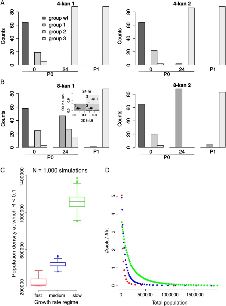
Figure 2.
Population structure of evolving populations. (A) E. coli populations grown in 4-kan are more homogeneous in composition and comprised mostly of fit variants at 24 h. Isolates were classified into several groups based on the stationary-phase OD600 reached in 4-kan (tolerance to kanamycin) and 0-kan (growth in the absence of kanamycin; see inset in B). Plotted are counts of different types of isolates. Wild-type-like isolates (black bars) have been arbitrarily defined for the analysis as non-tolerant but fit isolates (falling in the OD range indicated in the inset of B) and predominate at the start of the experiment (0 h.). Group 1 (dark grey) isolates are tolerant but sick variants. Group 2 (grey) and 3 (light grey) are tolerant and fit variants (see inset of Figure 1B for definition of groups based on stationary-phase OD600 in plain LB and 4-kan and Supplementary Figure S5 for all plots related to this figure as well as plots for 0-kan control populations in which the wild-type-like colonies predominate throughout the course of the experiment). The counts change with time during the course of the batch evolution experiment (0 h, 24 h and P1). Results of the first replicate are displayed in the left panel and the second replicate in the right panel. (B) Populations grown in 8-kan are composed of multiple subpopulations, with the sick variants dominating at 24 h. Thus, tolerant but sick variants predominate in the first batch growth in 8-kan, and subsequent passaging results in an increase in number of the fit variants. (C) 1,000 independent growth simulations were performed for three growth regimes. This plot shows the distributions of the total population size (a reflection of the number of iterations or time) at which the ratio of the sick mutant to the fit mutant falls below 10%. Distributions are represented by box plots. The box represents the inter-quartile range and the line within the box indicates the median value. The maximum and the minimum value (1.5 times the inter-quartile range), excluding the outliers, is represented by the whiskers. The points represent the outliers. Probabilities of division per iteration are as follows. For the slow growth regime (green), µwt = 0.01, µsick = 0.03 and µfit = 0.1; for the intermediate growth regime (blue), µwt = 0.03, µsick = 0.1 and µfit = 0.3; for the fast growth regime (red), µwt = 0.1, µsick = 0.3 and µfit = 1. (D) A scatter plot of the ratio of the number of sick to fit mutants as a function of the population size (equivalent to the number of iterations or time) for an example simulation from (C).

