Localized Principal Component Analysis based Curve Evolution: A Divide and Conquer Approach

Abstract

We propose a novel localized principal component analysis (PCA) based curve evolution approach which evolves the segmenting curve semi-locally within various target regions (divisions) in an image and then combines these locally accurate segmentation curves to obtain a global segmentation. The training data for our approach consists of training shapes and associated auxiliary (target) masks. The masks indicate the various regions of the shape exhibiting highly correlated variations locally which may be rather independent of the variations in the distant parts of the global shape. Thus, in a sense, we are clustering the variations exhibited in the training data set. We then use a parametric model to implicitly represent each localized segmentation curve as a combination of the local shape priors obtained by representing the training shapes and the masks as a collection of signed distance functions. We also propose a parametric model to combine the locally evolved segmentation curves into a single hybrid (global) segmentation. Finally, we combine the evolution of these semilocal and global parameters to minimize an objective energy function. The resulting algorithm thus provides a globally accurate solution, which retains the local variations in shape. We present some results to illustrate how our approach performs better than the traditional approach with fully global PCA.

1. Introduction

Level set based shape prior models are widely used in various computer vision applications like segmentation, tracking, shape recognition to obtain prior knowledge from training data. Principal component analysis (PCA) is commonly used to generate shape priors. In this paper, we focus our attention on one such application, a localized PCA based shape prior implementation for image segmentation.

The concept of using prior shape knowledge for segmentation was introduced by Cootes et al. in [5]. Later Chen et al. [4] used average shape in a geometric active contour model and Leventon et al. [8] used a level set framework to restrict the flow of active contours using shape information. Level set based shape prior models for image segmentation were developed later in [9, 11]. Cremers et al. [6] developed a method to improve segmentation by selectively preferring certain shape priors/objects over others. Davatzikos et al. [7] showed that using wavelets in a Hierarchical Active Shape Model framework can capture certain local variations. Recently authors in [12] developed an explicit ASM-based scheme that generates independent partitions and uses PCA strictly local to these partitions and authors in [1] use fully global PCA with weighted local fitting. All the above-mentioned approaches treat the entire shape as a single global entity.

In our paper, we develop the concept of using localized shape priors for segmentation. We first divide our image domain into various target regions by clustering parts of the global shape which exhibit highly-correlated local shape variations. The variations in these regions may be independent of the variations in other parts of the global shape. We can use these local shape priors in an explixit curve representation framework, as in the case with the Active Shape Models, or we can use these shape priors in an implicit level set based shape prior approach. In this paper, we develop local PCA-based shape priors in a level set framework, but our approach can be extended to the explicit ASM scheme by following a similar procedure.

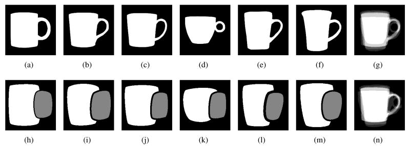
Figure 1 shows a sample set of training images. These images are manual segmentations of the objects we intend to segment, mugs in this case. The target masks shown in Figure 1(h-m) separate the variations in the shape of the handle from the shape of the body of the mug.

Figure 1.

(a-f) Training images, (h-m) Target Masks: The white regions mark Target Mask ‘1’ - capturing variations in the shape of the body. Gray regions mark Target Mask ‘2’ - capturing variations in the shape of the handle. (g) Shape overlay before alignment (n) Shape overlay after alignment.

With these target regions, we use a spatially weighted (local) PCA [10] to learn the shape variation in each target region. Thus, we focus the learning from PCA to these regions and maximize the utility of each principal component (shape prior). Since we use a spatially weighted learning and fitting procedure, we do not require very precise target masks.

We represent our training shapes and target masks using the level set formulation described in [11]. We apply local PCA on the level sets for the shape and the mask to obtain a set of eigenshapes (shape priors) and eigenmasks (mask priors) corresponding to each target mask. We can then represent the segmenting curve and the mask for each (target) semi-local segmentation as a linear combination of these local eigenshapes and eigenmasks. Evolving the curves locally within these masks generates locally accurate segmentation curves. We combine these curves to obtain a hybrid global segmentation curve. Finally, we evolve this hybrid curve to obtain a globally accurate segmentation.

Although the semi-local parameters affect the global shape of the segmenting curve, their evolution depends on information local to the mask. Henceforth, in the paper, we will refer to these semi-local parameters and semi-local segmentation curves as local parameters and local segmentation curves, respectively. In Sections 3 and 4, we discuss the procedure for using local shape priors for segmentation. In Section 5, we explain the combined evolution of various local segmentation curves. Finally, in Section 6, we use our approach for Myocardial segmentation in cardiac images.

2. Binary Shape Alignment

It is standard procedure to align the training images before using PCA. This ensures that the priors will capture only the shape variations and not the pose variations. Consider a training data set with n images, {I₁, I₂, …, I_n}. For each 2D image I_i, we also define a pose parameter vector p_i, such that p = [a, b, h, θ], where a, b, h and θ represent the x-, y-translation, scale and rotation, respectively. We jointly align the n images in our training set by minimizing the following energy functional [11] with respect to the pose parameters:

$$E_{\mathit{\text{align}}}=\sum _{i=1}^n\sum _{j=1,j\ne i}^n\left\{\frac{\underset{\mathrm{\Omega }}{\int }\int {({\stackrel{\sim }{I}}^i-{\stackrel{\sim }{I}}^j)}^2\mathit{\text{dA}}}{\underset{\mathrm{\Omega }}{\int }\int {({\stackrel{\sim }{I}}^i+{\stackrel{\sim }{I}}^j)}^2\mathit{\text{dA}}}\right\},$$ (1)

where the transformed image of I is denoted by Ĩ. Since the target masks correspond to regions in the original training images, we do not align the target masks separately. Instead, we transform the masks with the same set of pose parameters obtained by aligning the training shapes. In Figure 1(g) and 1(n), we show an overlay of training images before and after alignment.

3. Local Shape Priors

We use signed distance functions to represent the shapes and the masks [8, 9, 11]. The zero level set depicts the shape/mask boundary, with positive distances indicating the regions inside the boundary and negative distances indicating the regions outside the boundary. Let {ψ₁, ψ₂, …ψ_n} denote the signed distance functions for the n shapes and {φ_T1, φ_T2, …φ_Tn} denote the signed distance functions for the corresponding binary masks for a specific target T. The mean level set for the shapes, $\overline{\Psi }=(1/n){\sum }_{i=1}^n{\Psi }_i,$and the mean level set for the masks of a given target T is ${\overline{\varphi }}_T=(1/n){{\sum }_{i=1}^n\varphi }_{Ti}$. Now, we define an extended shape variability matrix for each target mask as explained in [2].

$$S_T=\left(\right[\begin{array}{c}{\Psi }_1-\overline{\Psi }\\ {\varphi }_{T1}-{\overline{\varphi }}_T\end{array}]\left[\begin{array}{c}{\Psi }_2-\overline{\Psi }\\ {\varphi }_{T2}-{\overline{\varphi }}_T\end{array}\right]\dots \left[\begin{array}{c}{\Psi }_n-\overline{\Psi }\\ {\varphi }_{Tn}-{\overline{\varphi }}_T\end{array}\right])\cdot$$ (2)

In addition to the shape variability matrix we also define a weighting matrix M_T, for each target T,

$$M_T=\left(\right[\begin{array}{c}g({\varphi }_{T1})\\ \mathbf{1}\end{array}]\left[\begin{array}{c}g({\varphi }_{T2})\\ \mathbf{1}\end{array}\right]\dots \left[\begin{array}{c}g({\varphi }_{Tn})\\ \mathbf{1}\end{array}\right]).$$

Here g(·) is a non-linear function which has unit weight for the elements within the mask and for the regions outside the mask it monotonically decreases to zero as we move away from the boundary of the mask (g(ϕ̃ ≥ 0) = 1, 0 < g(ϕ̃ < 0) < 1). 1 denotes unit weight for elements which correspond to the mask. Now, we use spatially weighted EM framework [10] to estimate k principal components for shape and target mask (k < n). The matrix M_T gives higher emphasis to the regions within the mask, hence the shape priors will capture the local variations better. We denote the localized principal components for the shapes and masks as {ψ̂_T1, ψ̂_T2, …ψ̂_Tk} and {ϕ̂_T1, ϕ̂_T2, …ϕ̂_Tk}, respectively.

We now formulate a new level set function, ψ̃_T, as a linear combination of the mean level set (ψ̄) and the k principal modes (local shape priors). In addition to the k modes, we also have to accommodate the pose variations in the framework. For a given target mask T, we define the new level sets for shape and mask as

$${\stackrel{\sim }{\Psi }}_T(\mathbf{\alpha },{\mathbf{p}}_{\mathbf{T}})=\overline{\Psi }({\mathbf{p}}_{\mathbf{T}})+\sum _{l=1}^k{\alpha }_{Tl}{\widehat{\Psi }}_{Tl}({\mathbf{p}}_{\mathbf{T}}),$$ (3)

$${\stackrel{\sim }{\varphi }}_T(\mathbf{\alpha },{\mathbf{p}}_{\mathbf{T}})=\overline{\varphi }({\mathbf{p}}_{\mathbf{T}})+\sum _{l=1}^k{\alpha }_{Tl}{\widehat{\varphi }}_{Tl}({\mathbf{p}}_{\mathbf{T}}).$$ (4)

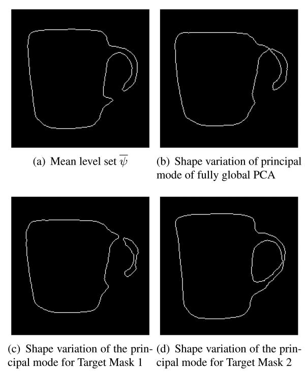
Here p_T is the pose vector and {α_T1, α_T2, …, α_Tl} are the weights associated with principal modes {ψ_T1, ψ_T2, …, ψ_Tl} and {ϕ_T1,ϕ_T2, …,ϕ_Tl}. The zero level set of ψ̃ represents the shape boundary and by varying the weights α_T, we can vary the shape implicitly. The evolution of the ϕ̃ should correspond to evolution of ψ̃. Thus, we use the same set of pose and shape parameters for both ψ̃ and ϕ̃. Figure 2 compares the variation caused by the principal mode of fully global PCA with the variation caused by the principal modes of the local PCA for the two target masks.

Figure 2.

Shape variability of fully global PCA and localized PCA.

4. Local Parameter Optimization via Gradient Descent

In this section, we describe the coupled evolution of ψ̃ and ϕ̃ to segment the region of an image within the given target mask. The domain under consideration will not be the entire image, but only the region within the mask (ϕ̃ ≥ 0). We need to choose a geometric active contour energy model to segment this region. In this paper, we use region-based energy, although other forms of energies may also be used effectively. Consider a general class of region-based energy

$$E(\stackrel{\sim }{\Psi },\stackrel{\sim }{\varphi })={\int }_{R^{\mathit{\text{in}}}}{f}_{\mathit{\text{in}}}(x,y)\mathit{\text{dA}}+{\int }_{R^{\mathit{\text{out}}}}{f}_{\mathit{\text{out}}}(x,y)\mathit{\text{dA}},$$ (5)

where $R^{\mathit{\text{in}}}=\{(x,y)\in {ℝ}^2:\stackrel{\sim }{\Psi }(x,y)<0,\stackrel{\sim }{\varphi }(x,y)\ge 0\}$and $R^{\mathit{\text{out}}}=\{(x,y)\in {ℝ}^2:\stackrel{\sim }{\Psi }(x,y)\ge 0,\stackrel{\sim }{\varphi }(x,y)\ge 0\}$.

We employ gradient descent on E(ψ̃, ϕ̃) with respect to the pose parameters p and shape parameters α_l for the evolution of ψ̃. For concise notations, we denote Θ as a collective representation of the pose and shape parameters. We denote the gradient of E(ψ̃, ϕ̃) with respect to a given parameter Θ by ∇_ΘE. The update equation for parameter Θ is given by

$${\Theta }^{i+1}={\Theta }^i‒\nabla {}_{\Theta }E\mathit{\text{dt}}.$$

We now denote the zero level set of ψ̃ and ϕ̃ by C_ψ̃ and C_ϕ̃, respectively. The evolution of parameters Θ results in the evolution of ψ̃ and ϕ̃, which causes an implicit evolution of C_ψ̃ and C_ϕ̃. Figure 3 shows a graphical representation of ψ̃ and ϕ̃. To compute ∇_ΘE, we need the line integral on the curve C. We can thus represent ∇_ΘE as the line integral

Figure 3.

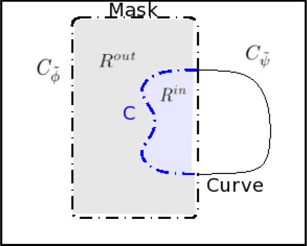
Domain under consideration is marked by the shaded region. The region inside the mask and the curve form Rⁱⁿ and the region outside the curve but inside the mask forms R^out.

$$\nabla {}_{\Theta }E=\underset{C}{\int }{f}_{\mathit{\text{in}}}\nabla {}_{\Theta }C{\overrightarrow{N}}_{\stackrel{\sim }{\Psi }}\mathit{\text{ds}}+\underset{C}{\int }{f}_{\mathit{\text{out}}}\nabla {}_{\Theta }C(-{\overrightarrow{N}}_{\stackrel{\sim }{\Psi }})ds,$$ (6)

where s is the arc length parameter of the curve and N⃗ _ψ̃ is the outward normal of the zero level set of ψ̃.

Since the zero level set of ψ̃ is a function of C and Θ, we have

$$\stackrel{\sim }{\Psi }(C(\Theta ,s),\Theta )=0.$$ (7)

Taking the gradient of (7) w.r.t. Θ, we get

$$\begin{array}{c}{\nabla }_{\Theta }\stackrel{\sim }{\Psi }+\nabla \stackrel{\sim }{\Psi }\cdot {\nabla }_{\Theta }C=0\hfill \\ \Rightarrow {\nabla }_{\Theta }\stackrel{\sim }{\Psi }+\parallel \nabla \stackrel{\sim }{\Psi }\parallel \cdot {\overrightarrow{N}}_{\stackrel{\sim }{\Psi }}\cdot {\nabla }_{\Theta }C=0\hfill \\ \Rightarrow {\nabla }_{\Theta }C\cdot {\overrightarrow{N}}_{\stackrel{\sim }{\Psi }}=\frac{-{\nabla }_{\Theta }\stackrel{\sim }{\Psi }}{\parallel \nabla \stackrel{\sim }{\Psi }\parallel }\cdot \hfill \end{array}$$ (8)

Substituting (8) in Equation (6), we get

$${\nabla }_{\Theta }E=\underset{C}{\int }(\frac{-{\nabla }_{\Theta }\stackrel{\sim }{\Psi }}{\parallel \nabla \stackrel{\sim }{\Psi }\parallel })(f_{\mathit{\text{in}}}-f_{\mathit{\text{out}}})\mathit{\text{ds}},$$ (9)

where ${\overrightarrow{N}}_{\stackrel{\sim }{\Psi }}=\frac{\nabla \stackrel{\sim }{\Psi }}{\parallel \nabla \stackrel{\sim }{\Psi }\parallel }$.

In the examples presented here, we use the region-based energy functional proposed by Chan and Vese [3]. Thus, we use the following choices for functions f_in and f_out:

$$f_{\mathit{\text{in}}}={(I-\mu )}^2,f_{\mathit{\text{out}}}={(I-v)}^2,$$

where μ and ν denote the mean intensity values inside the regions R_in and R_out respectively.

Figure 4 shows an example of local segmentation using two target masks. We initialize the segmentation with the mean level set shown in Figure 2(a). Since the curve evolves only on the basis of the cues within the mask, we get a reliable segmentation in the regions inside the mask.

Figure 4.

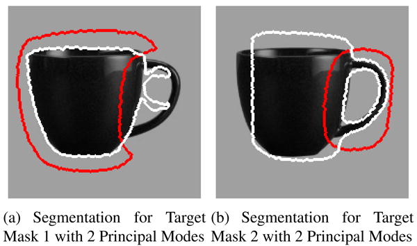
Local segmentation: Red curves mark the boundary of the target mask. The segmentation is accurate inside each target mask (without caring for the segmentation outside the mask).

5. Combined Shape Evolution

5.1. Initialization

The target regions are chosen such that they isolate correlated local variations. In reality, the local variations in the various target regions are never completely independent. Thus, we have to combine the local segmentation curves corresponding to each target mask to obtain a hybrid segmentation. To combine the individual local segmentation curves we use the same level set framework that we used in generating the local segmentation.

Given N target regions, we combine the level sets {ψ̃₁, ψ̃₂, …ψ̃_N} into a single hybrid level set Ψ_init.

$${\mathrm{\Psi }}_{\mathit{\text{init}}}=\frac{{\sum }_{T=1}^N\{{\lambda }_T\rho ({\stackrel{\sim }{\varphi }}_T)\cdot {\stackrel{\sim }{\Psi }}_T({\mathbf{\alpha }}_T,{\mathbf{p}}_T)\}}{{\sum }_{T=1}^N\{{\lambda }_T\rho ({\stackrel{\sim }{\varphi }}_T)\}},$$ (10)

where λ_T is the scalar weight associated with each target level set and ρ(ϕ̃_T) ≥ 0 is a non-linear function. We set the value of λ_T = 1/N to obtain the initial hybrid level set. The function ρ(·) should be 1 in the regions within the mask (positive values of ϕ̃_T and for the regions outside the mask it should monotonically decrease to zero as we move away from the mask boundary. In the regions where the masks overlap, the hybrid level set will be the average of the overlapping level sets. Thus, the hybrid level set seamlessly combines the various target level sets (with a higher weight given to the regions inside each mask).

5.2. Evolution

Along with the k principal modes corresponding to each target level set ψ̃_T, we use a single set of pose parameters P for the hybrid level set Ψ. Since we have a new set of pose parameters, we will update the eigenshapes and eigenmasks for each target with the corresponding pose parameters (ψ̂_Tl = ψ̂_Tl(p_T), ϕ̂_Tl = ϕ̂_Tl(p_T)). Thus, (3) becomes

$${\stackrel{\sim }{\Psi }}_T({\mathit{A}}_T,\mathbf{P})={\mathrm{\Psi }}_{\mathit{\text{init}}}(\mathbf{P})+\sum _{l=1}^k{A}_{Tl}{\hat{\Psi }}_{Tl}(\mathbf{P}),$$ (11)

where A_T are the weights associated with the new eigenshapes. A similar equation can be derived for the update of the mask ϕ̃_T. Now, we can express the hybrid level set as

$$\mathrm{\Psi }=\frac{{\sum }_{T=1}^N\{{\lambda }_T\rho ({\stackrel{\sim }{\varphi }}_T)\cdot {\stackrel{\sim }{\Psi }}_T({\mathit{A}}_T,\mathbf{P})\}}{{\sum }_{T=1}^N\{{\lambda }_T\rho ({\stackrel{\sim }{\varphi }}_T)\}}\cdot$$ (12)

This hybrid level set is a function of the set of pose parameters (P), shape parameters corresponding to each target region {A₁, A₂, …, A_N} and scalar weights {λ₁, λ₂, …, λ_N}. We converge to the final segmentation by employing gradient descent (Section 4) on each of these parameters. The parameters λ_T and A_T will evolve based on the cues within their respective target regions. Thus, the evolution still retains the local properties within each mask. But the pose parameters will be affected by the collective region of all the target masks, hence the pose parameters evolve based on global cues. Thus, the final segmentation retains the local shape variations in each mask and these variations are combined using global pose parameters.

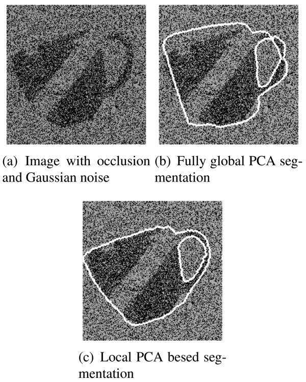
Figure 5(a) shows the final evolved hybrid segmentation using 2 principal modes for each target mask. Figure 5(b) shows the segmentation obtained using the fully global PCA approach using 4 principal modes. Although we use the same number of principal modes to segment the image in both cases, the local PCA approach does a very good job of capturing the shape of the body of the mug as well as the handle. Since most of the effort from the fully global PCA is used in learning and fitting the shape of the body, it is unable to segment the handle correctly. Our approach concentrates the efforts of the local PCA to segment each target region separately, thus achieving a better global segmentation. In Figure 6, we show results on the same test image with added occlusions, variation in pose and additive Gaussian noise. These results suggest that our approach is robust under such demanding conditions, which are common to various segmentation tasks.

Figure 5.

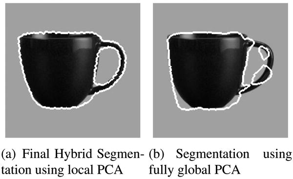
The final hybrid segmentation successfully segments the handle and the body of the mug, where as the fully global PCA approach uses all its training resources to capture the variation in the mug body and fails to segment the handle.

Figure 6.

Segmentation on mug image with occlusion and noise.

6. Application to Cardiac Image Segmentation

Myocardial segmentation in cardiac images is considered a very challenging problem because of the low contrast separating the ventricles from the myocardium and partially missing boundaries along the ventricles. In our experiment, we used a data set of 200 2-D images from a 4-D interactive manual segmentation of a single patient's cardiac CT scan. We used 100 of these images for training and the test set consisted the other 100 images. Figure 7 shows an example of one training image slice with the corresponding manual segmentation. To generate the masks we dilate the left and right ventricles from the manual tracing. We dilate the masks enough to include some parts from the exterior regions of the epicardial boundary.

Figure 7.

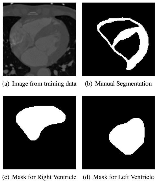
Myocardial Segmentation: Training data and masks.

Figure 8 compares the results of segmentation on a test image. We use 12 principal modes for each target mask, and compare our result with the fully global PCA approach with 24 principal modes. Our approach segments the boundaries along both the ventricles and the epicardium, whereas the fully global PCA approach tries to fit the curve simultaneously on the endocardial and epicardial boundary, and in the process fails to achieve either. We note that the masks were generated automatically from the training data, which suggests that our approach does not rely on custom designed masks. The masks need not be designed accurately; any mask that can successfully cluster the correlated local shape variations will improve segmentation. Since our approach uses fewer modes for segmentation, it can be very useful in cases where the training data set consists limited data.

Figure 8.

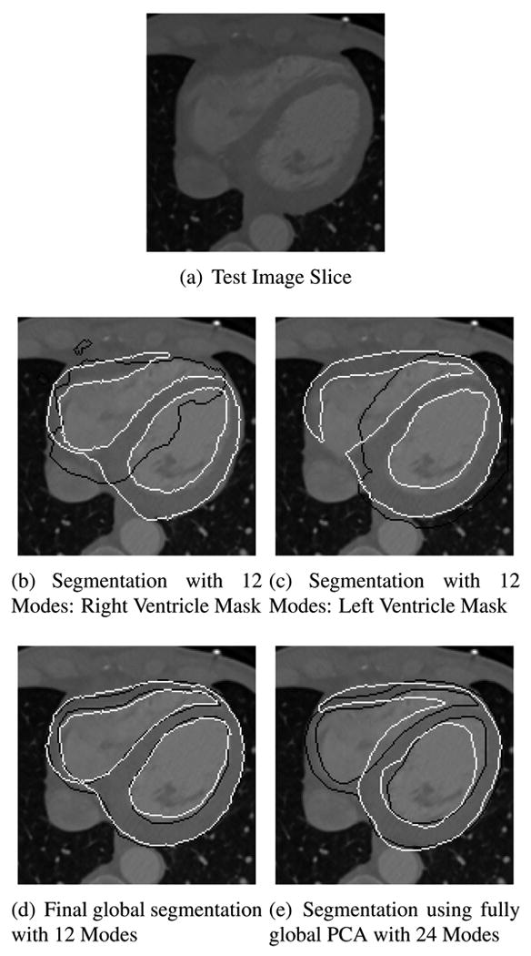
(a) Cardiac image (b,c) Black curve - boundary of target mask, White curve - semi-local segmentation. (d,e) Black curve -manual tracing, White curve - Final Segmentation. (d,e) Average distance between the manual tracing and segmentation: (d) (1.47 ± 1.88)mm. (e) (5.21 ± 6.41)mm.

7. Conclusion

We have presented a variational framework that can employ local shape priors to segment within various target regions in an image and then combine these locally accurate segmentation curves to obtain a single globally accurate segmentation. The examples presented in our paper show that concentrating the efforts of the local shape priors within certain target regions can enhance the utility of PCA as a tool.

References

- 1.Amberg M, Luthi M, Vetter T. Local regression based statistical model fitting. Proceedings of the 32nd DAGM conference on Pattern recognition; 2010. pp. 452–461. [Google Scholar]
- 2.Appia VV, Ganapathy B, Abufadel A, Yezzi A, Faber T. A regions of confidence based approach to enhance segmentation with shape priors. Computational Imaging, SPIE. 2010;7533(1) doi: 10.1117/12.850888. [DOI] [PMC free article] [PubMed] [Google Scholar]
- 3.Chan TF, Vese LA. A level set algorithm for minimizing the mumford-shah functional in image processing. IEEE workshop on variational and level set methods in computer vision. 2001:161. [Google Scholar]
- 4.Chen Y, Thiruvenkadam S, Huang F, Wilson D, Geiser EA, Tagare HD. On the incorporation of shape priors into geometric active contours. Variational and level set methods in computer vision. 2001:145. [Google Scholar]
- 5.Cootes TF, Taylor CJ, Cooper DH, Graham J. Active shape models - their training and application. Computer vision image understanding. 1995;61:38–59. [Google Scholar]
- 6.Cremers D, Sochen N, Schnörr C. Multiphase dynamic labeling for variational recognition-driven image segmentation. IJCV. 2006;66:67–81. [Google Scholar]
- 7.Davatzikos C, Tao X, Shen D. Hierarchical active shape models, using the wavelet transform. Transactions of Medical Iamging. 2003 Mar;22(3):414–423. doi: 10.1109/TMI.2003.809688. [DOI] [PubMed] [Google Scholar]
- 8.Leventon M, Grimson E, Faugeras O. Statistical shape influence in geodesic active contours. CVPR. 2000;1:316–323. [Google Scholar]
- 9.Rousson M, Paragios N. Shape priors for level set representations. ECCV. 2002:78–92. [Google Scholar]
- 10.Skočaj D, Leonardis A, Bischof H. Weighted and robust learning of subspace representations. Pattern recognition. 2007;40(5):1556–1569. [Google Scholar]
- 11.Tsai A, Yezzi A, Wells W, Tempany C, Tucker D, Fan A, Grimson WE, Willsky A. A shape-based approach to the segmentation of medical imagery using level sets. IEEE transactions on medical imaging. :137–154. doi: 10.1109/TMI.2002.808355. [DOI] [PubMed] [Google Scholar]
- 12.Zhao Z, Aylward S, Teoh E. A novel 3D partitioned active shape model for segmentation of brain MR images. MICCAI 2005. 2005:221–228. doi: 10.1007/11566465_28. [DOI] [PubMed] [Google Scholar]