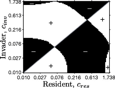
Fig. 6.

Pairwise invasibility plot. The axes are the c value for the resident (horizontal) and the invader (vertical), and the regions are indicated by whether the invader invades (white region with plus sign) or not (black region with minus sign). We followed the outline of the technique in Klausmeier et al. (2007) for invasion in a model with forced fluctuations. Beginning near the stable limit cycle of the resident, we introduced invaders at small biomass with the same s. Invasion success was calculated by comparing maximum invader biomass from the first half of the simulation time to the second half. Simulation time after introducing the invader varied from four to 500 fluctuation periods. Longer periods were necessary near the transitions because some invading types initially decreased in biomass (see Electronic Supplementary Materials). Input fluctuations occurred over a period 32π. Other parameters are as in Table 1 except for μ ₀ (0.03), ψ (0.006), and γ (0.02). Types with c > 1.738 for these parameters go extinct. The figure shows two locally stable points—c → 0 and intermediate c—separated by an evolutionary repellor. The intermediate c is also globally stable: It invades any type and cannot be invaded by any type